Plots to Stands: Producing LiDAR Vegetation Metrics for Imputation Calculations

Some professionals in remote sensing find LAStools a useful tool to extract statistical metrics from LiDAR that are used to make estimations about a larger area of land from a small set of sample plots. Common applications are prediction of the timber volume or the above-ground biomass for entire forests based on a number of representative plots where exact measurements were obtained with field work. The same technique can also be used to make estimations about animal habitat or coconut yield or to classify the type of vegetation that covers the land. In this tutorial we describe the typical workflow for computing common metrics for smaller plots and larger areas using LAStools.

Download these six LiDAR tiles (1, 2, 3, 4, 5, 6) from a Eucalyptus plantation in Brazil to follow along the step by step instructions of this tutorial. This data is courtesy of Suzano Pulp and Paper. Please also download the two shapefiles that delineate the plots where field measurements were taken and the stands for which predictions are to be made. You should download version 170327 (or higher) of LAStools due to some recent bug fixes.

Quality Checking

Before processing newly received LiDAR data we always perform a quality check first. This ranges from visual inspection with lasview, to printing textual content reports and attribute histograms with lasinfo, to flight-line alignment checks with lasoverlap, pulse density and pulse spacing checks with lasgrid and las2dem, and completeness-of-returns check with lassort followed by lasreturn.

lasinfo -i tiles_raw\CODL0003-C0006.laz ^
        -odir quality -odix _info -otxt

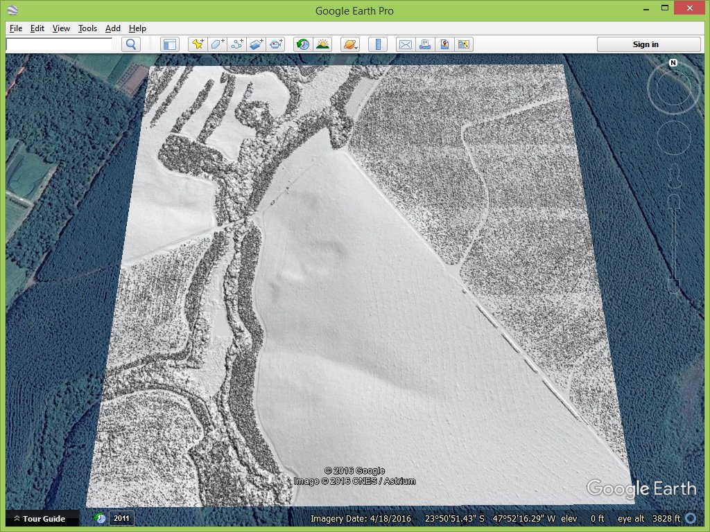
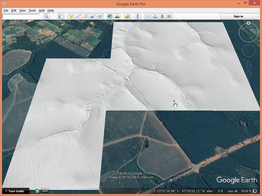
The lasinfo report tells us that there is no projection information. However, we remember that this Brazilian data was in the common SIRGAS 2000 projection and try for a few likely UTM zones whether the hillshaded DSM produced by las2dem falls onto the right spot in Google Earth.

las2dem -i tiles_raw\CODL0003-C0006.laz ^
        -keep_first -thin_with_grid 1 ^
        -hillshade -epsg 31983 ^
        -o epsg_check.png

The lasinfo report also tells us that the xyz coordinates are stored with millimeter resolution which is a bit of an overkill. For higher and faster LASzip compression we will later lower this to a more appropriate centimeter resolution. It further tells us that the returns are stored using point type 0 and that is a bit unfortunate. This (older) point type does not have a GPS time stamp so that some quality checks (e.g. „completeness of returns“ with lasreturn) and operations (e.g. „resorting of returns into acquisition order“ with lassort) will not be possible. Fortunately the min-max range of the ‚point source ID‘ suggests that this point attribute is correctly populated with flightline numbers so that we can do a check for overlap and alignment of the different flightlines that contribute to the LiDAR in each tile.

lasoverlap -i tiles_raw\*.laz ^
           -min_diff 0.2 -max_diff 0.4 ^
           -epsg 31983 ^
           -odir quality -opng ^
           -cores 3

We run lasoverlap to visualize the amount of overlap between flightlines and the vertical differences between them. The produced images (see below) color code the number of flightlines and the maximum vertical difference between any two flightlines as seen below. Most of the area is cyan (2 flightlines) except in the bottom left where the pilot was sloppy and left some gaps in the yellow seams (3 flightlines) so that some spots are only blue (1 flightline). We also see that two tiles in the upper left are partly covered by a diagonal flightline. We will drop that flightline later to create a more uniform density.across the tiles. The mostly blue areas in the difference are mostly aligned with features in the landscape and less with the flightline pattern. Closer inspection shows that these vertical difference occur mainly in the dense old growth forests with species of different heights that are much harder to penetrate by the laser than the uniform and short-lived Eucalyptus plantation that is more of a „dead forest“ with little undergrowth or animal habitat.

Interesting observation: The vertical difference of the lowest return from different flightlines computed per 2 meter by 2 meter grid cell could maybe be used a new forestry metric to help distinguish mono cultures from natural forests.

lasgrid -i tiles_raw\*.laz ^
        -keep_last ^
        -step 2 -point_density ^
        -false -set_min_max 10 20 ^
        -epsg 31983 ^
        -odir quality -odix _d_2m_10_20 -opng ^
        -cores 3

lasgrid -i tiles_raw\*.laz ^
        -keep_last ^
        -step 5 -point_density ^
        -false -set_min_max 10 20 ^
        -epsg 31983 ^
        -odir quality -odix _d_5m_10_20 -opng ^
        -cores 3

We run lasgrid to visualize the pulse density per 2 by 2 meter cell and per 5 by 5 meter cell. The produced images (see below) color code the number of last return per square meter. The impact of the tall Eucalyptus trees on the density per cell computation is evident for the smaller 2 meter cell size in form of a noisy blue/red diagonal in the top right as well as a noisy blue/red area in the bottom left. Both of those turn to a more consistent yellow for the density per cell computation with larger 5 meter cells. Immediately evident is the higher density (red) for those parts or the two tiles in the upper left that are covered by the additional diagonal flightline. The blueish area left to the center of the image suggests a consistently lower pulse density whose cause remains to be investigated: Lower reflectivity? Missing last returns? Cloud cover?

The lasinfo report suggests that the tiles are already classified. We could either use the ground classification provided by the vendor or re-classify the data ourselves (using lastile, lasnoise, and lasground). We check the quality of the ground classification by visually inspecting a hillshaded DTM created with las2dem from the ground returns. We buffer the tiles on-the-fly for a seamless hillshade without artifacts along tile boundaries by adding ‚-buffered 25‘ and ‚-use_orig_bb‘ to the command-line. To speed up reading the 25 meter buffers from neighboring tiles we first create a spatial indexing with lasindex.

lasindex -i tiles_raw\*.laz ^
         -cores 3

las2dem -i tiles_raw\*.laz ^
        -buffered 25 ^
        -keep_class 2 -thin_with_grid 0.5 ^
        -use_orig_bb ^
        -hillshade -epsg 31983 ^
        -odir quality -odix _dtm -opng ^
        -cores 3

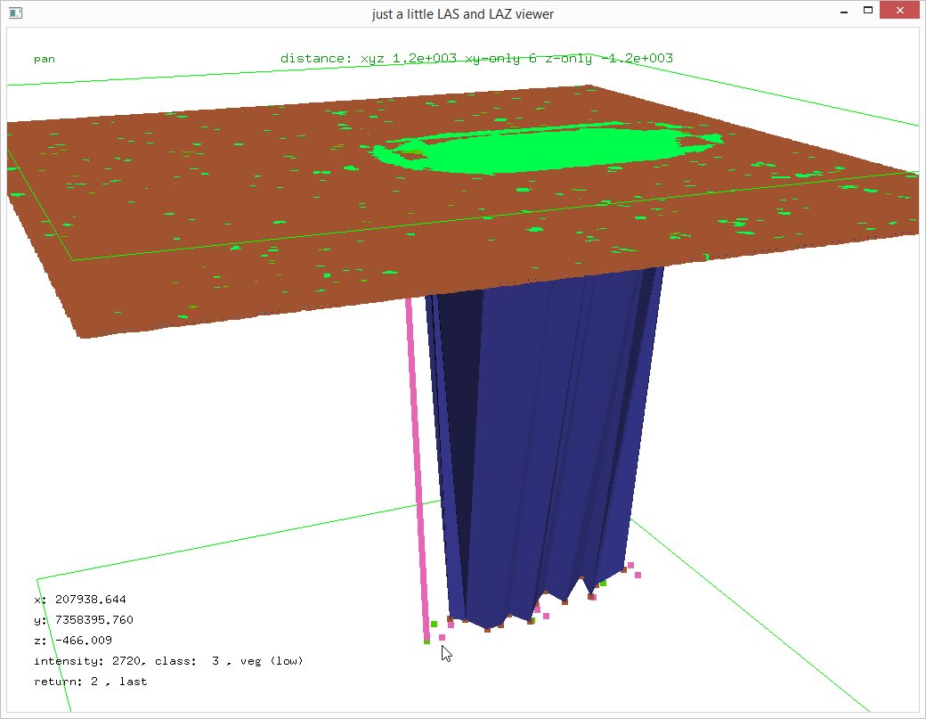
The resulting hillshaded DTM shows a few minor issues in the ground classification but also a big bump (above the mouse cursor). Closer inspection of this area (you can cut it from the larger tile using the command-line below) shows that there is a group of miss-classified points about 1200 meters below the terrain. Hence, we will start from scratch to prepare the data for the extraction of forestry metrics.

las2las -i tiles_raw\CODL0004-C0006.laz ^
        -inside_tile 207900 7358350 100 ^
        -o bump.laz

lasview -i bump.laz

Data Preparation

Using lastile we first tile the data into smaller 500 meter by 500 meter tiles with 25 meter buffer while flagging all points in the buffer as ‚withheld‘. In the same step we lower the resolution to centimeter and put nicer a coordinate offset in the LAS header. We also remove the existing classification and classify all points that are much lower than the target terrain as class 7 (aka noise). We also add CRS information and give each tile the base name ’suzana.laz‘.

lastile -i tiles_raw\*.laz ^
        -rescale 0.01 0.01 0.01 ^
        -auto_reoffset ^
        -set_classification 0 ^
        -classify_z_below_as 500.0 7 ^
        -tile_size 500 ^
        -buffer 25 -flag_as_withheld ^
        -epsg 31983 ^
        -odir tiles_buffered -o suzana.laz

With lasnoise we mark the many isolated points that are high above or below the terrain as class 7 (aka noise). Using two tiles we played around with the ’step‘ parameters until we find good parameter settings. See the README of lasnoise for the exact meaning and the choice of parameters for noise classification. We look at one of the resulting tiles with lasview.

lasnoise -i tiles_buffered\*.laz ^
         -step_xy 4 -step_z 2 ^
         -odir tiles_denoised -olaz ^
         -cores 3

lasview -i tiles_denoised\suzana_206000_7357000.laz ^
        -color_by_classification ^
        -win 1024 192

Next we use lasground to classify the last returns into ground (2) and non-ground (1). It is important to ignore the noise points with classification 7 to avoid the kind of bump we saw in the vendor-delivered classification. We again check the quality of the computed ground classification by producing a hillshaded DTM with las2dem. Here the las2dem command-line is sightly different as instead of buffering on-the-fly we use the buffers stored with each tile.

lasground -i tiles_denoised\*.laz ^
          -ignore_class 7 ^
          -nature -extra_fine ^
          -odir tiles_ground -olaz ^
          -cores 3

las2dem -i tiles_ground\*.laz ^
        -keep_class 2 -thin_with_grid 0.5 ^
        -hillshade ^
        -use_tile_bb ^
        -odir quality -odix _dtm_new -opng ^
        -cores 3

Finally, with lasheight we compute how high each return is above the triangulated surface of all ground returns and store this height value in place of the elevation value into the z coordinate using the ‚-replace_z‘ switch. This height-normalizes the LiDAR in the sense that all ground returns are set to an elevation of 0 while all other returns get an elevation relative to the ground. The result are height-normalized LiDAR tiles that are ready for producing the desired forestry metrics.

lasheight -i tiles_ground\*.laz ^
          -replace_z ^
          -odir tiles_normalized -olaz ^
          -cores 3

Metric Production

The tool for computing the metrics for the entire area as well as for the individual field plots is lascanopy. Which metrics are well suited for your particular imputation calculation is your job to determine. Maybe first compute a large number of them and then eliminate the redundant ones. Do not use any point from the tile buffers for these calculations. We had flagged them as ‚withheld‘ during the lastile operation, so they are easy to drop. We also want to drop the noise points that were classified as 7. And we were planning to drop that additional diagonal flightline we noticed during quality checking. We generated two lasinfo reports with the ‚-histo point_source 1‘ option for the two tiles it was covering. From the two histograms it was easy to see that the diagonal flightline has the number 31.

First we run lascanopy on the 11 plots that you can download here. When running on plots it makes sense to first create a spatial indexing with lasindex for faster querying so that only those tiny parts of the LAZ file need to be loaded that actually cover the plots.

lasindex -i tiles_normalized\*.laz ^
         -cores 3

lascanopy -i tiles_normalized\*.laz -merged ^
          -drop_withheld ^
          -drop_class 7 ^
          -drop_point_source 31 ^
          -lop WKS_PLOTS.shp ^
          -cover_cutoff 3.0 ^
          -cov -dns ^
          -height_cutoff 2.0 ^
          -c 2.0 999.0 ^
          -max -avg -std -kur ^
          -p 25 50 75 95 ^
          -b 30 50 80 ^
          -d 2.0 5.0 10.0 50.0 ^
          -o plots.csv

The resulting ‚plots.csv‘ file you can easily process in other software packages. It contains one line for each polygonal plot listed in the shapefile that lists its bounding box followed by all the requested metrics. But is why is there a zero maximum height (marked in orange) for plots 6 though 10? All height metrics are computed solely from returns that are higher than the ‚height_cutoff‘ that was set to 2 meters. We added the ‚-c 2.0 999.0‘ absolute count metric to keep track of the number of returns used in these calculations. Apparently in plots 6 though 10 there was not a single return above 2 meters as the count (also marked in orange) is zero for all these plots. Turns out this Eucalyptus stand had recently been harvested and the new seedlings are still shorter than 2 meters.

more plots.csv
index,min_x,min_y,max_x,max_y,max,avg,std,kur,p25,p50,p75,p95,b30,b50,b80,c00,d00,d01,d02,cov,dns
0,206260.500,7358289.909,206283.068,7358312.477,11.23,6.22,1.91,2.26,4.71,6.01,7.67,9.5,26.3,59.7,94.2,5359,18.9,41.3,1.5,76.3,60.0
1,206422.500,7357972.909,206445.068,7357995.477,13.54,7.5,2.54,1.97,5.32,7.34,9.65,11.62,26.9,54.6,92.2,7030,12.3,36.6,13.3,77.0,61.0
2,206579.501,7358125.909,206602.068,7358148.477,12.22,5.72,2.15,2.5,4.11,5.32,7.26,9.76,46.0,73.7,97.4,4901,24.8,28.7,2.0,66.8,51.2
3,206578.500,7358452.910,206601.068,7358475.477,12.21,5.68,2.23,2.64,4.01,5.14,7.18,10.04,48.3,74.1,95.5,4861,25.7,26.2,2.9,68.0,50.2
4,206734.501,7358604.910,206757.068,7358627.478,15.98,10.3,2.18,2.64,8.85,10.46,11.9,13.65,3.3,27.0,91.0,4946,0.6,32.5,44.5,91.0,77.5
5,207043.501,7358761.910,207066.068,7358784.478,15.76,10.78,2.32,3.43,9.27,11.03,12.49,14.11,3.2,20.7,83.3,4819,1.5,24.7,51.0,91.1,76.8
6,207677.192,7359630.526,207699.760,7359653.094,0.00,0.00,0.00,0.00,0.00,0.00,0.00,0.00,0.0,0.0,0.0,0,0.0,0.0,0.0,0.0,0.0
7,207519.291,7359372.366,207541.859,7359394.934,0.00,0.00,0.00,0.00,0.00,0.00,0.00,0.00,0.0,0.0,0.0,0,0.0,0.0,0.0,0.0,0.0
8,207786.742,7359255.850,207809.309,7359278.417,0.00,0.00,0.00,0.00,0.00,0.00,0.00,0.00,0.0,0.0,0.0,0,0.0,0.0,0.0,0.0,0.0
9,208159.017,7358997.344,208181.584,7359019.911,0.00,0.00,0.00,0.00,0.00,0.00,0.00,0.00,0.0,0.0,0.0,0,0.0,0.0,0.0,0.0,0.0
10,208370.909,7358602.565,208393.477,7358625.133,0.00,0.00,0.00,0.00,0.00,0.00,0.00,0.00,0.0,0.0,0.0,0,0.0,0.0,0.0,0.0,0.0

Then we run lascanopy on the entire area and produce one raster per tile for each metric. Here we remove the buffered points with the ‚-use_tile_bb‘ switch that also ensures that the produced rasters have exactly the extend of the tiles without buffers. Again, it is imperative that you download the version 170327 (or higher) of LAStools for this to work correctly.

lascanopy -version
LAStools (by martin@rapidlasso.com) version 170327 (academic)

lascanopy -i tiles_normalized\*.laz ^
          -use_tile_bb ^
          -drop_class 7 ^
          -drop_point_source 31 ^
          -step 10 ^
          -cover_cutoff 3.0 ^
          -cov -dns ^
          -height_cutoff 2.0 ^
          -c 2.0 999.0 ^
          -max -avg -std -kur ^
          -p 25 50 75 95 ^
          -b 30 50 80 ^
          -d 2.0 5.0 10.0 50.0 ^
          -odir tile_metrics -oasc ^
          -cores 3

The resulting rasters in ASC format can easily be previewed using lasview for some „sanity checking“ that our metrics make sense and to get a quick overview about what these metrics look like.

lasview -i tile_metrics\suzana_*max.asc
lasview -i tile_metrics\suzana_*p95.asc
lasview -i tile_metrics\suzana_*p50.asc
lasview -i tile_metrics\suzana_*p25.asc
lasview -i tile_metrics\suzana_*cov.asc
lasview -i tile_metrics\suzana_*d00.asc
lasview -i tile_metrics\suzana_*d01.asc
lasview -i tile_metrics\suzana_*b30.asc
lasview -i tile_metrics\suzana_*b80.asc

The maximum height rasters are useful to inspect more closely as they will immediately tell us if there was any high noise point that slipped through the cracks. And indeed it happened as we see a maximum of 388.55 meters for of the 10 by 10 meter cells. As we know the expected height of the trees we could have added a ‚-drop_z_above 70‘ to the lascanopy command line. Careful, however, when computing forestry metrics in strongly sloped terrains as the terrain slope can significantly lift up returns to heights much higher than that of the tree. This is guaranteed to happen for LiDAR returns from branches that are extending horizontally far over the down-sloped part of the terrain as shown in this paper here.

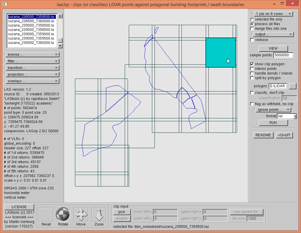
We did not use the shapefile for the stands in this exercise. We could have clipped the normalized LiDAR points to these stands using lasclip as shown in the GUI below before generating the raster metrics. This would have saved space and computation time as many of the LiDAR points lie outside of the stands. However, it might be better to do that clipping step on the rasters in whichever GIS software or statistics package you are using for the imputation computation to properly account for partly covered raster cells along the stand boundary. This could be subject of another blog article … (-: