A while back we had a first look at the Single Photon LiDAR from Leica’s SPL100 sensor (that eventually turned out just to be an SPL99 because one beamlet or one receiver in the 10 by 10 array was broken and did not produce any returns). Today we are taking a closer look at a strategy to remove the excessive noise in the raw Single Photon LiDAR data from a „proper“ SPL100 sensor (where all of the 100 beamlets are firing) that was flown in 2017 in Navarra, Spain.

The data was provided as open data by the cartography section of Navarra’s Government and is available via a simple download FTP portal. We describe the LAStools processing steps that were used to eliminate the excessive noise and to generate a smooth DTM. In the following we are using the originally released version of the data, that we obtained shortly after the portal went online that seems to be a bit more „raw“ than the current files available now. One starndard quality check with lasinfo was done with:
lasinfo -i 0_raw\*.laz ^
        -cd ^
        -histo intensity 1 ^
        -histo user_data 1 ^
        -histo point_source 1 ^
        -histo gps_time 10 ^
        -odir 1_quality -odix _info -otxt
Upon inspecting the lasinfo report we suggest a few changes in how to store this Single Photon LiDAR data for more efficient hosting via an online portal. We perform these changes here before starting the actual processing. First we use the las2las call shown below to fix an error in the global encoding bits, remove an irrelevant VLR, re-scale the coordinates from millimeter to centimeters, re-offset the coordinates to nice numbers, and – what is by far the most crucial change for better compression – remap the beamlet ID stored in the ‚user data‘ field as described in an earlier article.
las2las -i 0_raw\*.laz ^
        -rescale 0.01 0.01 0.01 ^
        -auto_reoffset ^
        -set_global_encoding_gps_bit 1 ^
        -remove_vlr 1 ^
        -map_user_data beamlet_ID_map.txt ^
        -odir 2_fix_rescale_reoffset_remap -olaz ^
        -cores 3
Then we use two lassort calls, one to maximize compression and one to improve spatial coherence. One lassort call rearranges the points in increasing order first based on the GPS time stamps, then breaks ties based on the user data field (that stores the beamlet ID), and finally stores the returns of every beamlet ordered by return number. We also add spatial reference information in this step. The other lassort call rearranges the points into a spatially coherent layout. It uses a Z-order sort with the granularity of 50 meter by 50 meter buckets of points. Within each bucket the point order from the prior sort is kept.
lassort -i 2_fix_rescale_reoffset_remap\*.laz ^
        -epsg 25830 ^
        -gps_time ^
        -user_data ^
        -return_number ^
        -odir 2_maximum_compression -olaz ^
        -cores 3

lassort -i 2_maximum_compression\*.laz ^
        -bucket_size 50 ^
        -odir 2_spatial_coherence -olaz ^
        -cores 3
The resulting optimized nine tiles are around 200 MB each and can be downloaded as one file here or as individual tiles here:
- las_ca_544_4710_2017_NAV_EPSG25830.laz
- las_ca_544_4711_2017_NAV_EPSG25830.laz
- las_ca_544_4712_2017_NAV_EPSG25830.laz
- las_ca_545_4710_2017_NAV_EPSG25830.laz
- las_ca_545_4711_2017_NAV_EPSG25830.laz
- las_ca_545_4712_2017_NAV_EPSG25830.laz
- las_ca_546_4710_2017_NAV_EPSG25830.laz
- las_ca_546_4711_2017_NAV_EPSG25830.laz
- las_ca_546_4712_2017_NAV_EPSG25830.laz
Now we start the usual processing workflow by tiling the data with lastile into smaller 500 meter by 500 meter tiles with a 25 meter buffer. We also set the pre-existing point classification in the data to zero as we will compute our own later.
lastile -i 2_spatial_coherence\*.laz ^
        -set_classification 0 ^
        -tile_size 500 -buffer 25 -flag_as_withheld ^
        -odir 3_buffered -o yecora.laz
We notice that a large amount of the noise has intensity values below 1000. We are still a bit puzzled where those intensity values come from and what exactly they mean in a Single Photon LiDAR system. But it works. We run las2las with a „filtered transform“ to set classification of all points whose intensity value is 1000 or less to the classification code 7 (aka „noise“).
las2las -i 3_buffered\*.laz ^
        -keep_intensity_below 1000 ^
        -filtered_transform ^
        -set_classification 7 ^
        -odir 4_intensity_denoised -olaz ^
        -cores 3
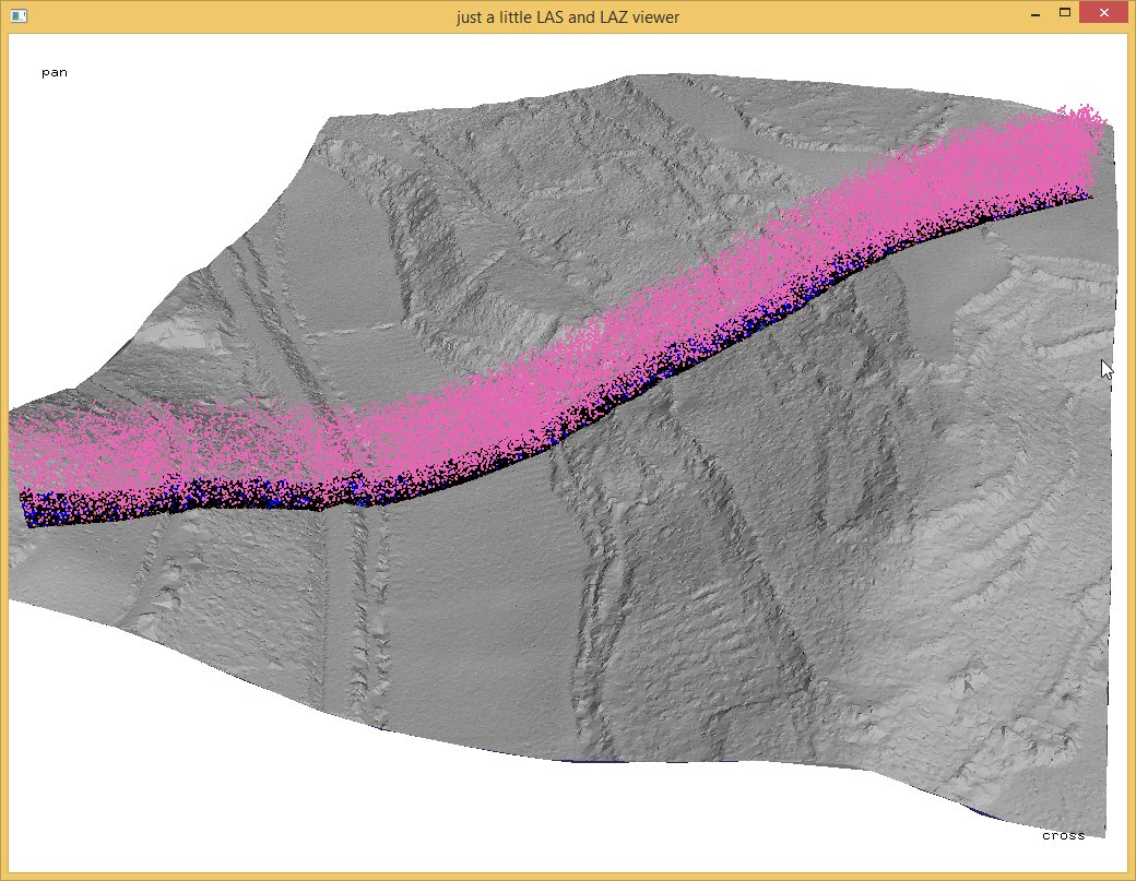
We then ignore this „easy-to-identify“ noise and go after the remaining one with lasnoise by ignoring classification code 7 and setting the newly identified noise to classification code 9 – not because it’s „water“ (the usual meaning of class 9) but because these points are drawn with a distinct blue color when checking the result with lasview.
 lasnoise -i 4_intensity_denoised\*.laz ^
         -ignore_class 7 ^
         -step_xy 1.0 -step_z 0.2 ^
         -isolated 5 ^
         -classify_as 9 ^
         -odir 4_isolation_denoised -olaz ^
         -cores 3
Of the surviving non-noise points we then use lasthin to reclassify the point closest to the 20th elevation percentile per 50 cm by 50 cm area with classification code 8 (for all areas that have more than 5 non-noise points per 50 cm by 50 cm area. We repeat the same for every 1 meter by 1 meter area.
lasthin -i 4_isolation_denoised\*.laz ^
        -ignore_class 7 9 ^
        -step 0.5 -percentile 20 5 ^
        -classify_as 8 ^
        -odir 5_thinned_p20_050cm -olaz ^
        -cores 3

lasthin -i 5_thinned_p20_050cm\*.laz ^
        -ignore_class 7 9 ^
        -step 1.0 -percentile 20 5 ^
        -classify_as 8 ^
        -odir 5_thinned_p20_100cm -olaz ^
        -cores 3
We then perform a more agressive second noise removal step one with lasnoise using only those points with classification code 8, namely those non-noise points that were the 20th elevation percentile in either a 50 cm by 50 cm cell or a 1 meter by 1 meter cell. This can be done by ignoring classification code 0, 7, and 9. We mark those noise points as 6 so they appear orange in the point cloud with lasview.
lasnoise -i 5_thinned_p20_100cm\*.laz ^
         -ignore_class 0 7 9 ^
         -step_xy 2.0 -step_z 0.2 ^
         -isolated 1 ^
         -classify_as 6 ^
         -odir 5_thinned_p20_100cm_denoised -olaz ^
         -cores 3
The 20th elevation percentile points that survive the last noise removal are then classified into ground (2) and non-ground (1) points with lasground_new by ignoring all other points, namely those with classification codes 0, 6, 7, and 9.
lasground_new -i 5_thinned_p20_100cm_denoised\*.laz ^
              -ignore_class 0 6 7 9 ^
              -town ^
              -odir 5_tiles_ground_050cm -olaz ^
              -cores 3
These images below illustrate the steps we took. They also show that not all data was used and might give you ideas where to tweak our workflow for even better results.
Finally we raster the ground points into 1 meter Digital Terrain Model (DTM) rasters with las2dem and store the result (without buffers) to the RasterLAZ format.
las2dem -i 5_tiles_ground_050cm\*.laz ^
        -keep_class 2 ^
        -step 1.0 ^
        -use_tile_bb ^
        -odir 6_tiles_dtm_100cm -olaz ^
        -cores 3
Finally we merged all RasterLAZ tiles into one and compute the final hillshaded DTM with blast2dem.
blast2dem -i 6_tiles_dtm_100cm\*.laz -merged ^
          -step 1.0 ^
          -hillshade ^
          -o yecora_dtm_100cm.png
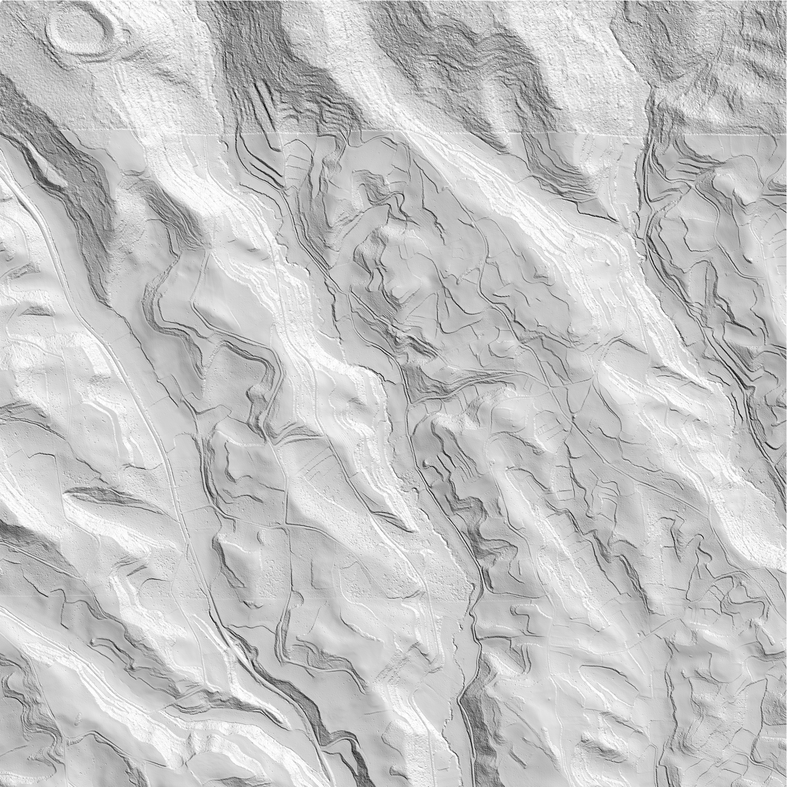
The hillshaded DTM that is result of the entire sequence of processing steps described above is shown below.

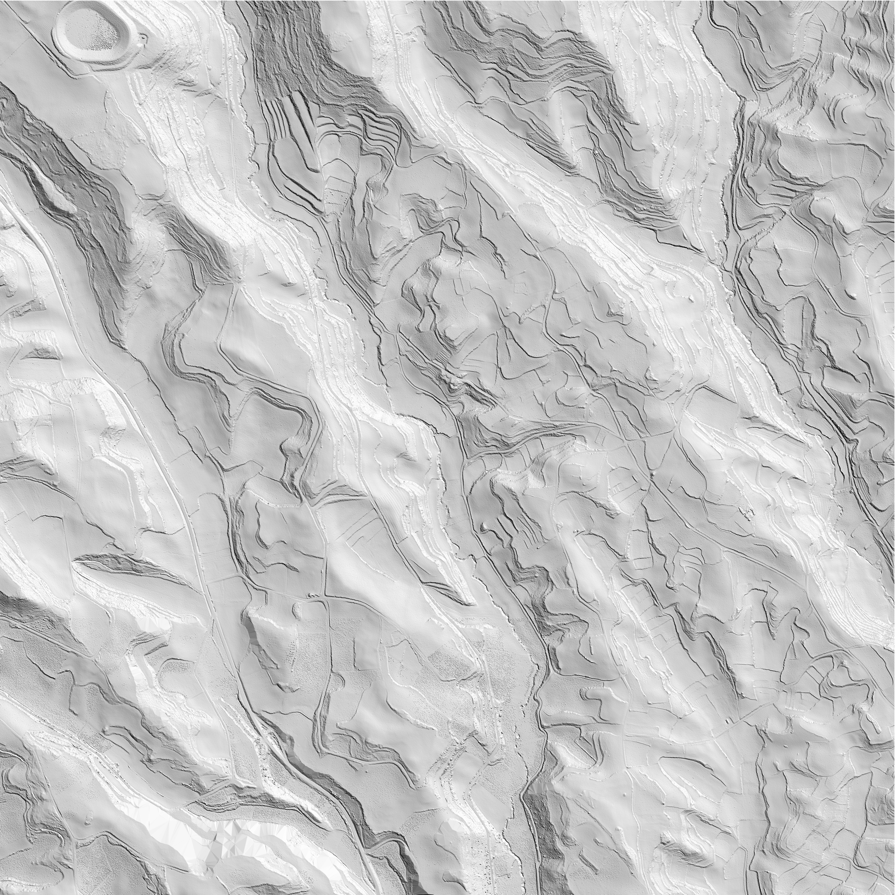
For comparison we generate the same DTM using the originally provided classification. According to the README file the original ground points are classified with code 22 in areas of flight line overlap and as the usual code 2 elsewhere. Hence we must use both classification codes to construct the DTM. We do this analogue to the earlier processing steps with the three LAStools commands lastile, las2dem, and blast2dem below.
lastile -i 2_spatial_coherence\*.laz ^
        -tile_size 500 -buffer 25 -flag_as_withheld ^
        -odir 3_tiles_buffered_orig -o yecora.laz

las2dem -i 3_tiles_buffered_orig\*.laz ^
        -keep_class 2 22 ^
        -step 1.0 ^
        -use_tile_bb ^
        -odir 6_tiles_dtm_100cm_orig -olaz ^
        -cores 3

blast2dem -i 6_tiles_dtm_100cm_orig\*.laz -merged ^
          -step 1.0 ^
          -hillshade ^
          -o yecora_dtm_100cm_orig.png
Below the hillshaded DTM generated from the ground classification that was provided with the LiDAR when it was originally released as open data.

In the meantime Andorra’s SPL data have been updated with a newer version in the open data portal. The new version of the data contains a much better ground classification that might have been improved manually as the new files now have the the string ‚cam‘ instead of ‚ca‘ in the file name, which probably means ‚classified automatically and manually‘ instead of the original ‚classified automatically‘. We decided not to switch to the new data release as it seemed less „raw“ than the original release. For example there are suddenly points with GPS times and returns counts and numbers of zero in the file that seem synthetic. But we also computed the hillshaded DTM for the new release which is shown below.

We thank the cartography section of Navarra’s Government for providing their LiDAR as open data. This not only allows re-purposing expensive data paid for by public taxes but also generates additional value, encourages citizen science, and provides educational opportunity and insights such as this blog article.
