You have guessed correctly. This is mostly fake news as our „Freistaat“ (read „Free State„) of Bavaria continues to tightly guard all of its tax-payer funded geospatial basis data for no good reason. Our other „Free State“ – that of Thuringia – has become one poster child of open data in Germany with North Rhine-Westphalia being the original one. But there is „some“ open LiDAR in Bavaria now.
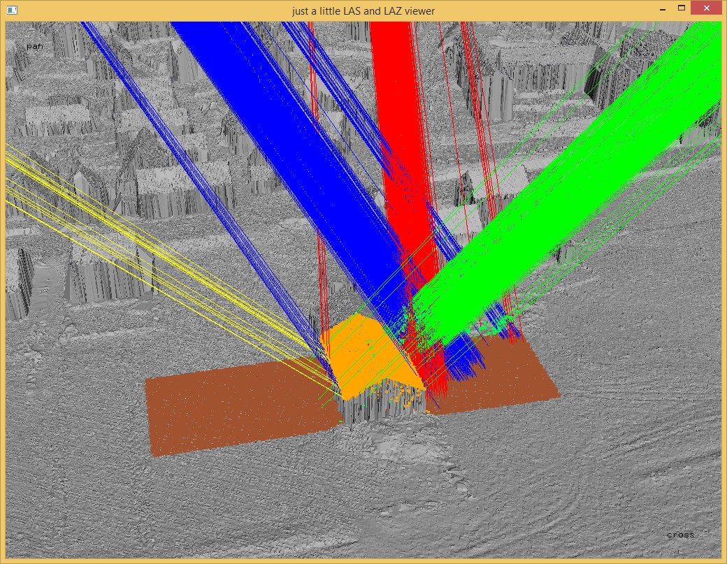
The authors of a recent paper on change detection in urban areas have published two interesting airborne LiDAR data sets from 2008 and 2009 for the town of Abenberg in [Hebel, Arens, Stilla, 2013]. What is interesting about these data sets is that they (a) were flown with a forward looking laser scanner with flight trajectories from 4 different directions (as illustrated in the image below) and (b) were surveyed again the same way in the following year for temporal change detection.

The data is provided for download here as zipped ASCII files that have one line per returns containing 11 comma-separated values. Below is a sample of the first 10 lines of the 2008 data:
1, 290.243, 28.663, -11.787, 0.060, -0.052, 0.997, 517.3170, -58.6934, 313.0817, 52
1, 290.208, 28.203, -11.825, 0.062, -0.056, 0.996, 517.3167, -58.6934, 313.0817, 49
1, 290.182, 27.739, -11.852, 0.063, -0.055, 0.997, 517.3164, -58.6935, 313.0817, 53
1, 290.165, 27.272, -11.866, 0.061, -0.058, 0.996, 517.3161, -58.6935, 313.0817, 53
1, 290.163, 26.800, -11.858, 0.061, -0.053, 0.997, 517.3157, -58.6935, 313.0817, 68
1, 290.152, 26.334, -11.864, 0.059, -0.054, 0.997, 517.3154, -58.6936, 313.0817, 57
1, 290.092, 25.882, -11.938, 0.050, -0.057, 0.997, 517.3151, -58.6936, 313.0817, 57
1, 290.103, 25.406, -11.911, 0.043, -0.058, 0.997, 517.3147, -58.6937, 313.0817, 63
1, 290.067, 24.947, -11.952, 0.043, -0.061, 0.997, 517.3144, -58.6937, 313.0817, 63
1, 290.034, 24.488, -11.989, 0.044, -0.063, 0.997, 517.3141, -58.6937, 313.0817, 56
The first number is either a classification into ground, vegetation, or other surface, or represents an identifier for a planar shape that the return is part of. The next three numbers in red are the x, y, and z coordinate of the LiDAR point in a local coordinate system. The next three numbers in green are the x, y, and z coordinates of an estimated surface normal. The next three numbers in blue are the x, y, and z coordinates of the sensor position. The last number is the intensity of the LiDAR return.
This textual representation makes it difficult to efficiently load the data into most LiDAR processing software. Also several attributes such as return number, number of returns, flight line ID, and GPS time stamps are missing.
We use this as an opportunity for a little exercise in converting ASCII to LAZ while preserving any „additional attributes“ using the „extra bytes“ functionality available since the LAS 1.4 specification. This is a timely experiment as the LAS Working Group of the ASPRS is currently contemplating how to standardize some useful „additional attributes“. Here you can download the resulting files:
- abenberg_data_2008.laz
- abenberg_data_2009.laz
In order to replicate these steps, please get your hands of the very latest version of LAStools. First we use txt2las to convert the TXT file to LAZ format as follows:
txt2las -i abenberg_data_2008.txt ^
        -set_point_type 1 ^
        -parse 0xyz123456i ^
        -set_scale 0.001 0.001 0.001 ^
        -add_attribute 3 "planar shape ID" "preliminary classification" ^
        -add_attribute 4 "normal x coord" "local normal direction estimate" 0.001 ^
        -add_attribute 4 "normal y coord" "local normal direction estimate" 0.001 ^
        -add_attribute 4 "normal z coord" "local normal direction estimate" 0.001 ^
        -add_attribute 6 "sensor x coord" "sensor position" 0.0001 ^
        -add_attribute 6 "sensor y coord" "sensor position" 0.0001 ^
        -add_attribute 6 "sensor z coord" "sensor position" 0.0001 ^
        -odix _temp1 -olaz
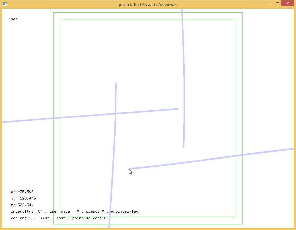
We use a back and forth of lasview and las2las with option ‚-subseq 12345 67890‘ to interactively find the exact index of the return where each flightline is ending and the next one is starting. The command below allows you to visualize the the trajectories.
lasview -i abenberg_data_2008_temp1.laz ^
        -copy_attribute_into_x 4 ^
        -copy_attribute_into_y 5 ^
        -copy_attribute_into_z 6 ^
        -points 10000000 ^
        -point_size 5

By hovering with the mouse over a point where the trajectory end and pressing ‚i‘ like info we can query the coordinates and attributes of a point. The console output also lists the index of the point in the file. We use this index as the start index for the manual search of the exact index where the flight lines really ends by piping the coordinates as text to stdout and looking for a „jump“ in coordinates that indicates the start of a new flightline as shown below.
las2las -i abenberg_data_2008_temp1.laz ^
        -subseq 1213485 1213505 ^
        -oparse xyz -otxt -stdout

-279.846 -98.442 -11.973
-279.984 -98.900 -12.123
-280.150 -99.357 -12.311
-280.195 -99.825 -12.332
-280.229 -100.294 -12.340
-280.275 -100.763 -12.363
-280.302 -101.233 -12.361
-280.344 -101.700 -12.379
-280.371 -102.171 -12.376
-280.156 -102.661 -12.042
110.259 304.077 3.873
110.646 304.118 3.925
111.036 304.154 3.970
111.424 304.167 3.982
111.811 304.211 4.037
112.201 304.252 4.088
112.588 304.278 4.118
112.976 304.315 4.164
113.364 304.336 4.186
113.752 304.344 4.192
Then we use the found index to seperate the first flight line form the rest with with two more runs of las2las:
las2las -i abenberg_data_2008_temp1.laz ^
         -subseq 0 1213495 ^
         -odix _strip1 -olaz

las2las -i abenberg_data_2008_temp1.laz ^
        -subseq 1213495 100000000 ^
        -odix _rest234 -olaz
We then repeat this procedure for the rest until we have four individual strips. Next we use las2las to change the point type from 0 to 1 to have a GPS time attribute that we will then populate with „fake“ but useful GPS time stamps:
las2las -i abenberg_data_2008_temp1_strip*.laz ^
        -set_point_type 1 ^
        -odix _pt1 -olaz
We noticed in the original text file that subsequent groups of points often have the exact same value for the three numbers in blue that are the x, y, and z coordinates of the sensor position. This suggests that those points are multiple returns from the same laser shot. We wrote a small tool using LASlib that exploits this observed pattern to recover the „return number“ and the „number of returns“ attribute for each point and to set a „fake“ but unique GPS time for each such group of returns. You can download the source code for this tool here. We run this tool for each strip with a different start GPS time:
lasrecover -i abenberg_data_2008_temp1_strip1_pt1.laz ^
           -gpstime_start 1000000 ^
           -odix _rec -olaz

lasrecover -i abenberg_data_2008_temp1_strip2_pt1.laz ^
           -gpstime_start 2000000 ^
           -odix _rec -olaz

lasrecover -i abenberg_data_2008_temp1_strip3_pt1.laz ^
           -gpstime_start 3000000 ^
           -odix _rec -olaz

lasrecover -i abenberg_data_2008_temp1_strip4_pt1.laz ^
           -gpstime_start 4000000 ^
           -odix _rec -olaz
Finally we merged the four strips back into one file using lasmerge:
lasmerge -i abenberg_data_2008_temp1_strip1_pt1_rec.laz ^
         -i abenberg_data_2008_temp1_strip2_pt1_rec.laz ^
         -i abenberg_data_2008_temp1_strip3_pt1_rec.laz ^
         -i abenberg_data_2008_temp1_strip4_pt1_rec.laz ^
         -faf ^
         -o abenberg_data_2008_temp2.laz
With lasview we are now able to visualize not only the multiple returns per shot but also the different angles from which the laser scanner has observed the scene.
Finally we use las2las and a „filtered transform“ with the custom classfication code provided in the first „additional attribute“ to populate the official LAS classification codes as ratified by the ASPRS. First we turn code 1 („Ground level“) into ground points.
las2las -i abenberg_data_2008_temp2.laz ^
        -keep_attribute_between 0 1 1 ^
        -filtered_transform ^
        -set_classification 2 ^
        -o abenberg_data_2008_temp3.laz
Then we turn code 5 („Vegetation“) into high vegetation points, code 6 („Other Surface“) into keypoints, and code 9 or higher („Planar shape #“) into building points.
las2las -i abenberg_data_2008_temp3.laz ^
        -keep_attribute_between 0 5 5 ^
        -filtered_transform ^
        -set_classification 5 ^
        -o abenberg_data_2008_temp4.laz

las2las -i abenberg_data_2008_temp4.laz ^
        -keep_attribute_between 0 6 6 ^
        -filtered_transform ^
        -set_classification 8 ^
        -o abenberg_data_2008_temp5.laz

las2las -i abenberg_data_2008_temp5.laz ^
         -keep_attribute_above 0 8 ^
         -filtered_transform ^
         -set_classification 6 ^
         -o abenberg_data_2008.laz
Then we are done. Here you can download the resulting files:
- abenberg_data_2008.laz
- abenberg_data_2009.laz
References
Hebel, M., Arens, M., Stilla, U., 2013. Change detection in urban areas by object-based analysis and on-the-fly comparison of multi-view ALS data. ISPRS Journal of Photogrammetry and Remote Sensing 86, pp. 52-64. [DOI: 10.1016/j.isprsjprs.2013.09.005] [PDF]

