This tutorial serves as an example for a complete end-to-end workflow that starts with raw LiDAR flightlines (as they may be delivered by a vendor) to final classified LiDAR tiles and derived products such as raster DTM, DSM, and SHP files with contours, building footprint and vegetation layers. The three example flightlines we are using here were flown in Ayutthaya, Thailand with a RIEGL LMS Q680i LiDAR scanner by Asian Aerospace Services who are based at the Don Mueang airport in Bangkok from where they are serving South-East-Asia and beyond. You can download them here:
- Ayutthaya_line_2.laz
- Ayutthaya_line_3.laz
- Ayutthaya_line_4.laz
Quality Checking
The minimal quality checks consist of generating textual reports (lasinfo & lasvalidate), inspecting the data visually (lasview), making sure alignment and overlap between flightlines fulfill expectations (lasoverlap), and measuring pulse density per square meter (lasgrid). Additional checks for points replication (lasduplicate), completeness of all returns per pulse (lasreturn), and validation against external ground control points (lascontrol) may also be performed.
lasinfo -i Ayutthaya\strips_raw\*.laz ^
        -cd ^
        -histo z 5 ^
        -histo intensity 64 ^
        -odir Ayutthaya\quality -odix _info -otxt ^
        -cores 3

lasvalidate -i Ayutthaya\strips_raw\*.laz ^
            -o Ayutthaya\quality\validate.xml
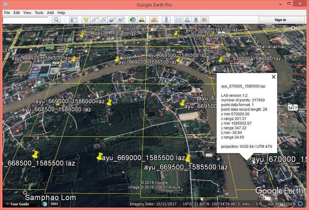
The lasinfo report generated with the command line shown computes the average density for each flightline and also generates two histograms, one for the z coordinate with a bin size of 5 meter and one for the intensity with a bin size of 64. The resulting textual descriptions are output into the specified quality folder with an appendix ‚_info‘ added to the original file name. Perusing these reports tells you that there are up to 7 returns per pulse, that the average pulse density per flightline is between 7.1 to 7.9 shots per square meter, that the point source IDs of the points are already populated correctly, that there are isolated points far above and far below the scanned area, and that the intensity values range from 0 to 1023 with the majority being below 400. The warnings in the lasinfo and the lasvalidate reports about the presence of return numbers 6 and 7 have to do with the history of the LAS format and can safely be ignored.
lasoverlap -i Ayutthaya\strips_raw\*.laz ^
           -files_are_flightlines ^
           -min_diff 0.1 -max_diff 0.3 ^
           -odir Ayutthaya\quality -o overlap.png
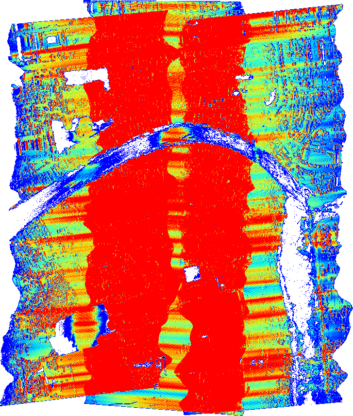
This results in two color illustrations. One image shows the flightline overlap with blue indicating one flightline, turquoise indicating two, and yellow indicating three flightlines. Note that wet areas (rivers, lakes, rice paddies, …) without LiDAR returns affect this visualization. The other image shows how well overlapping flightlines align. Their vertical difference is color coded with while meaning less than 10 cm error while saturated red and blue indicate areas with more than 30 cm positive or negative difference.


One pixel wide red and blue along building edges and speckles of red and blue in vegetated areas are normal. We need to look-out for large systematic errors where terrain features or flightline outlines become visible. If you click yourself through this photo album you will eventually see typical examples (make sure to read the comments too). One area slightly below the center looks suspicious. We load the PNG into the GUI to pick this area for closer inspection with lasview.
lasview -i Ayutthaya\strips_raw\*.laz -gui


Why these flightline differences exist and whether they are detrimental to your purpose are questions that you will have to explore further. For out purpose this isolated difference was noted but will not prevent us from proceeding further. Next we want to investigate the pulse density. We do this with lasgrid. We know that the average last return density per flightline is between 7.1 to 7.9 shots per square meter. We set up the false color map for lasgrid such that it is blue when the last return density drops to 5 shots (or less) per square meter and such that it is red when the last return density reaches 10 shots (or more).
lasgrid -i Ayutthaya\strips_raw\*.laz -merged ^
        -keep_last ^
        -step 2 -density ^
        -false -set_min_max 4 8 ^
        -odir Ayutthaya\quality -o density_4ppm_8ppm.png
The last return density image clearly shows how the density increases to over 10 pulses per square meter in all areas of flightline overlap. However, as there are large parts covered by only one flightline their density is the one that should be considered. We note great variations in density along the flightlines. Those have to do with aircraft movement and in particular with the pitch. When the nose of the plane goes up even slightly, the gigantic „fan of laser pulses“ (that can be thought of as being rigidly attached at the bottom perpendicular to the aircraft flight direction) is moving faster forward on the ground far below and therefore covers it with fewer shots per square meter. Conversely when the nose of the plane goes down the spacing between scan lines far below the plane are condensed so that the density increases. Inclement weather and the resulting airplane pitch turbulence can have a big impact on how regular the laser pulse spacing is on the ground. Read this article for more on LiDAR pulse density and spacing.
LiDAR Preparation
When you have airborne LiDAR in flightlines the first step is to tile the data into square tiles that are typically 1000 by 1000 or – for higher density surveys – 500 by 500 meters in size. This can be done with lastile. We also add a buffer of 30 meters to each tile. Why buffers are important for tile-based processing is explained here. We choose 30 meters as this is larger than any building we expect in this area and slightly larger than the ‚-step‘ size we use later when classifying the points into ground and non-ground points with lasground.
lastile -i Ayutthaya\strips_raw\*.laz ^
        -tile_size 500 -buffer 30 -flag_as_withheld ^
        -odir Ayutthaya\tiles_raw -o ayu.laz
NOTE: Usually you will have to add ‚-files_are_flightlines‘ or ‚-apply_file_source_ID‘ to the lastile command shown above in order to preserve the information which points is from which flightline. We do not have to do this here as evident from the lasinfo reports we generated earlier. Not only is the file source ID in the LAS header is correctly set to 2, 3, or 4 reflecting the intended flightline numbering evident from the file names. Also the point source ID of each point is already set to the correct value 2, 3, or 4. For more info see this or this discussion from the LAStools user forum.
Next we classify isolated points that are far from most other points with lasnoise into the (default) classification code 7. See the README file for the meaning of the parameters and play around with different setting to get a feel for how to make this process more or less aggressive.
lasnoise -i Ayutthaya\tiles_raw\ayu*.laz ^
         -step_xy 4 -step_z 2 -isolated 5 ^
         -odir Ayutthaya\tiles_denoised -olaz ^
         -cores 4
Especially for ground classification it is important that low noise points are excluded. You should inspect a number of tiles with lasview to make sure the low noise are all pink now if you color them by classification.
lasview -i Ayutthaya\tiles_denoised\ayu*.laz -gui
While the algorithms in lasground are designed to withstand a few noise points below the ground, you will find that it will include them into the ground model if there are too many of them. Hence, it is important to tell lasground to ignore these noise points. For the other parameters used see the README file of lasground.
lasground -i Ayutthaya\tiles_denoised\ayu*.laz ^
          -ignore_class 7 ^
          -city -ultra_fine ^
          -compute_height ^
          -odir Ayutthaya\tiles_ground -olaz ^
          -cores 4
You should visually check the resulting ground classification of each tile with lasview by selecting smaller subsets (press ‚x‘, draw a rectangle, press ‚x‘ again, use arrow keys to walk) and then switch back and forth between a triangulation of the ground points (press ‚g‘ and then press ‚t‘) and a triangulation of last returns (press ‚l‘ and then press ‚t‘). See the README of lasview for more information on those hotkeys.
lasview -i Ayutthaya\tiles_ground\ayu*.laz -gui
This way I found at least one tile that should be reclassified with ‚-metro‘ instead of ‚-city‘ because it still contained one large building in the ground classification. Alternatively you can correct miss-classifications manually using lasview as shown in the next few screen shots.


This is an optional step for advanced users who have a license. In case you managed to do such a manual edit and saved it as a LAY file using LASlayers (see the README file of lasview) you can overwrite the old file with:
laslayers -i Ayutthaya\tiles_ground\ayu_669500_1586500.laz -ilay ^
          -o Ayutthaya\tiles_ground\ayu_669500_1586500_edited.laz

move Ayutthaya\tiles_ground\ayu_669500_1586500_edit.laz ^
     Ayutthaya\tiles_ground\ayu_669500_1586500.laz
The next step classifies those points that are neither ground (2) nor noise (7) into building (or rather roof) points (class 6) and high vegetation points (class 5). For this we use lasclassify with the default parameters that only considers points that are at least 2 meters above the classified ground points (see the README for details on all available parameters).
lasclassify -i Ayutthaya\tiles_ground\ayu*.laz ^
            -ignore_class 7 ^
            -odir Ayutthaya\tiles_classified -olaz ^
            -cores 4
We check the classification of each tile with lasview by selecting smaller subsets (press ‚x‘, draw a rectangle, press ‚x‘ again) and by traversing with the arrow keys though the point cloud. You will find a number of miss-classifications. Boats are classified as buildings, water towers or complex temple roofs as vegetation, … and so on. You could use lasview to manually correct any classifications that are really important.
lasview -i Ayutthaya\tiles_classified\ayu*.laz -gui


Before delivering the classified LiDAR tiles to a customer or another user it is imperative to remove the buffers that were carried through all computations to avoid artifacts along the tile boundary. This can also be done with lastile.
lastile -i Ayutthaya\tiles_classified\ayu*.laz ^
        -remove_buffer ^
        -odir Ayutthaya\tiles_final -olaz ^
        -cores 4
Together with the tiling you may want to deliver a tile overview file in KML format (or in SHP format) that you can easily generate with lasboundary using this command line:
lasboundary -i Ayutthaya\tiles_final\ayu*.laz ^
            -use_bb ^
            -overview -labels ^
            -o Ayutthaya\tiles_overview.kml
Derivative production
The most common derivative product produced from LiDAR data is a Digital Terrain Model (DTM) in form of an elevation raster. This can be obtained by interpolating the ground points with a triangulation (i.e. a Delaunay TIN) and by sampling the TIN at the center of each raster cell. The pulse density of well over 4 shots per square meter definitely supports a resolution of 0.5 meter for the raster DTM. From the ground-classified tiles with buffer we compute the DTM using las2dem as follows:
las2dem -i Ayutthaya\tiles_ground\ayu*.laz ^
        -keep_class 2 ^
        -step 0.5 -use_tile_bb ^
        -odir Ayutthaya\tiles_dtm -obil ^
        -cores 4
It’s important to add ‚-use_tile_bb‘ to the command line which limits the raster generation to the original tile sizes of 500 by 500 meters in order not to rasterize the buffers that are extending the tiles 30 meters in each direction. We used the BIL format so that we inspect the resulting elevation rasters with lasview:
lasview -i Ayutthaya\tiles_dtm\ayu*.bil -gui
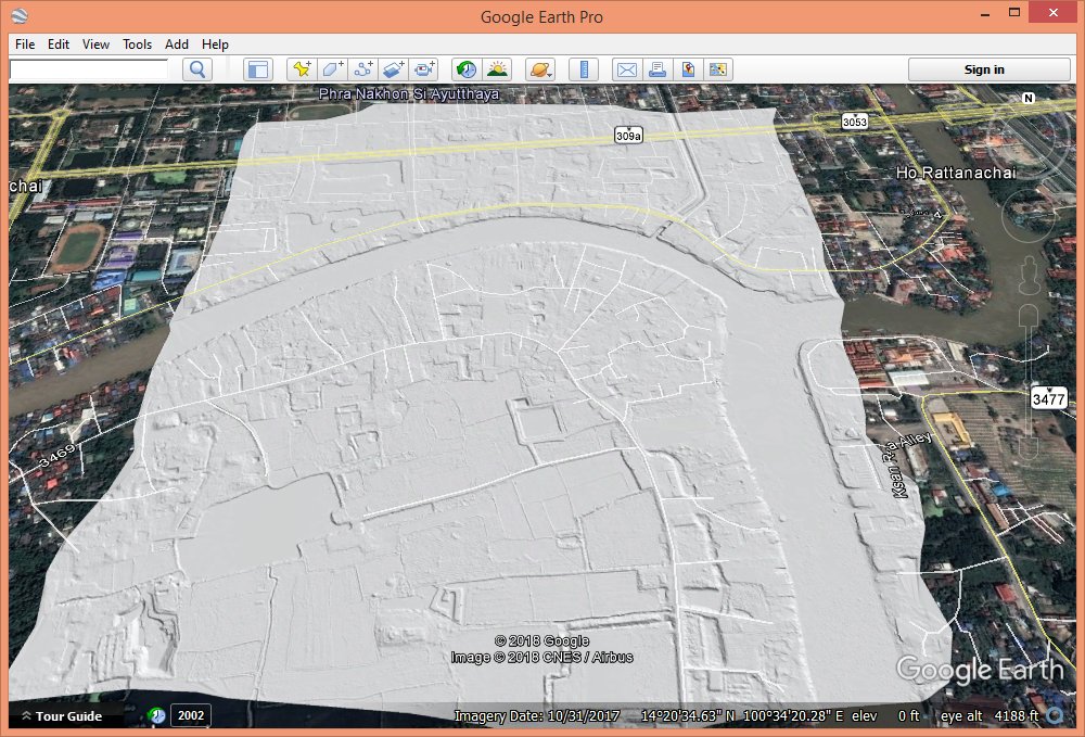
To create a hillshaded version of the DTM you can use your favorite raster processing package such as GDAL or GRASS but you could also use the BLAST extension of LAStools and create a large seamless image with blast2dem as follows:
blast2dem -i Ayutthaya\tiles_dtm\ayu*.bil -merged ^
          -step 0.5 -hillshade -epsg 32647 ^
          -o Ayutthaya\dtm_hillshade.png
Because blast2dem does not parse the PRJ files that accompany the BIL rasters we have to specify the EPSG code explicitly to also get a KML file that allows us to visualize the LiDAR in Google Earth.
Next we generate a Digital Surface Model (DSM) that includes the highest objects that the laser has hit. We use the spike-free algorithm that is implemented in las2dem that creates a triangulation of the highest returns as follows:
las2dem -i Ayutthaya\tiles_denoised\ayu*.laz ^
        -drop_class 7 ^
        -step 0.5 -spike_free 1.2 -use_tile_bb ^
        -odir Ayutthaya\tiles_dsm -obil ^
        -cores 4
We used 1.0 as the freeze value for the spike free algorithm because this is about three times the average last return spacing reported in the individual lasinfo reports generated during quality checking. Again we inspect the resulting rasters with lasview:
lasview -i Ayutthaya\tiles_dsm\ayu*.bil -gui
For reason of comparison we also generate the DSM rasters using a simple first-return interpolation again with las2dem as follows:
las2dem -i Ayutthaya\tiles_denoised\ayu*.laz ^
        -drop_class 7 -keep_first ^
        -step 0.5 -use_tile_bb ^
        -odir Ayutthaya\tiles_dsm -obil ^
        -cores 4
A few direct side-by-side comparison between a spike-free DSM and a first-return DSM shows the difference that are especially noticeable along building edges and in large trees.


Another product that we can easily create are building footprints from the automatically classified roofs using lasboundary. Because the tool is quite scalable we can simply on-the-fly merge the final tiles. This also avoids including duplicate points from the tile buffer whose classifications are also often less accurate.
lasboundary -i Ayutthaya\tiles_final\ayu*.laz -merged ^
            -keep_class 6 ^
            -disjoint -concavity 1.1 ^
            -o Ayutthaya\buildings.shp
Similarly we can use lasboundary to create a vegetation layer from those points that were automatically classified as high vegetation.
lasboundary -i Ayutthaya\tiles_final\ayu*.laz -merged ^
             -keep_class 5 ^
             -disjoint -concavity 3 ^
             -o Ayutthaya\vegetation.shp
We can also produce 1.0 meter contour lines from the ground classified points. However, for nicer contours it is beneficial to first generate a subset of the ground points with lasthin using option ‚-contours 1.0‘ as follows:
lasthin -i Ayutthaya\tiles_final\ayu*.laz ^
        -keep_class 2 ^
        -step 1.0 -contours 1.0 ^
        -odir Ayutthaya\tiles_temp -olaz ^
        -cores 4
We then merge all subsets of ground points from those temporary tiles on-the-fly into one (using the ‚-merged‘ option) and let blast2iso from the BLAST extension of LAStools generate smoothed and simplified 1 meter contours as follows:
blast2iso -i Ayutthaya\tiles_temp\ayu*.laz -merged ^
          -iso_every 1.0 ^
          -smooth 2 -simplify_length 0.5 -simplify_area 0.5 -clean 5.0 ^
          -o Ayutthaya\contours_1m.shp
Finally we composite all of our derived LiDAR products into one map using QGIS and then fuse it with data from OpenStreetMap that we’ve downloaded from BBBike. Here you can download the OSM data that we use.


It’s in particular interesting to compare the building footprints that were automatically derived from our LiDAR processing pipeline with those mapped by OpenStreetMap volunteers. We immediately see that there is a lot of volunteering work left to do and the LiDAR-derived data can assist us in directing those mapping efforts. A closer look reveals the (expected) quality difference between hand-mapped and auto-generated data.


The OSM buildings are simpler. These polygons are drawn and divided into logical units by a human. They are individually verified and correspond to actual buildings. However, they are less aligned with the Google Earth satellite image. The LiDAR-derived buildings footprints are complex because lasboundary has no logic to simplify the complicated polygonal chains that enclose the points that were automatically classified as roof into rectilinear shapes or to break directly adjacent roof points into separate logical units. However, most buildings are found (but also objects that are not buildings) and their geospatial alignment is as good as that of the LiDAR data.