Generating DTM for „fluffy“ Livox MID-40 LiDAR via „median ground“ points

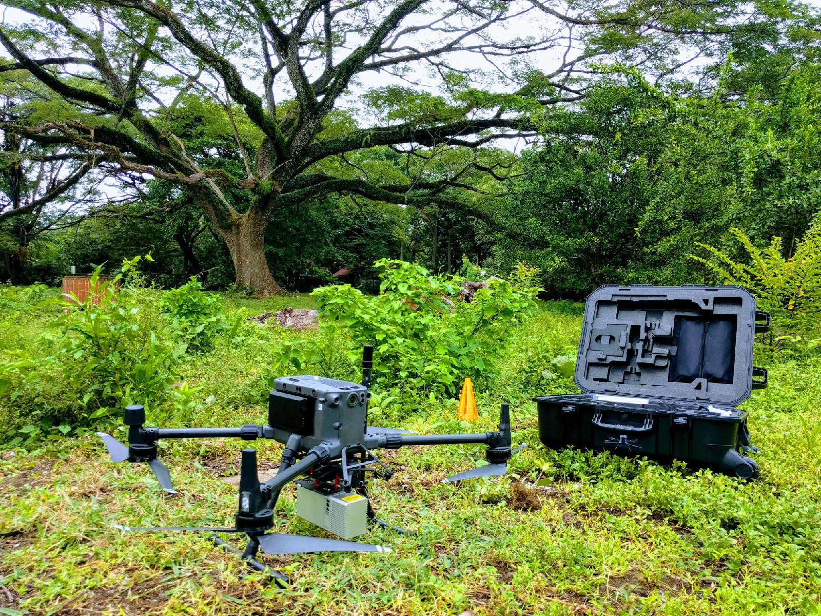
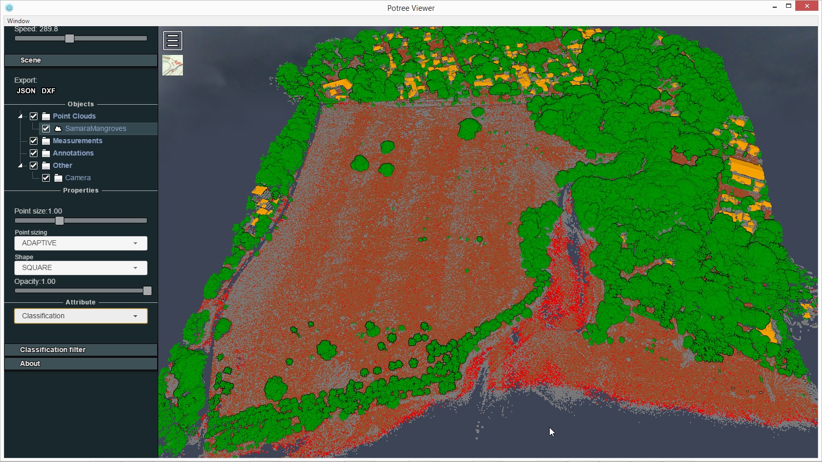
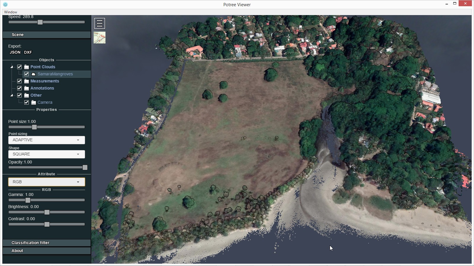
In the last article about the Livox MID-40 LiDAR scan of Samara we quality checked the data, aligned the flight lines and cleaned the remaining spurious scan lines. In this article we will process this data into the standard products. A focus will be on generating a smooth „median ground“ surface from the „fluffy“ scanner data. You can get the flight lines here and follow along with the processing after downloading LAStools. Below is one result of this work.

The first processing step will be to tile the strips into tiles that contain fewer points for faster and also parallel processing. One quick „flat terrain“ trick first. Often there are spurious points that are far above or below the terrain. For a relatively flat area these can be easily be identified by computing a histogram elevation values with lasinfo and then eliminated with simple drop-filters on the z coordinate.

lasinfo ^
-i Samara\Livox\03_strips_cleaned\*.laz ^
-merged ^
-histo z 1 ^
-odir Samara\Livox\01_quality ^
-o strips_cleaned_merged_info.txt

The relevant excerpts of the output of the lasinfo report are shown below:

[…]
z coordinate histogram with bin size 1.000000
bin -104 has 1
bin 5 has 1
bin 11 has 273762
bin 12 has 1387999
bin 13 has 5598767
bin 14 has 36100225
bin 15 has 53521371
[…]
bin 59 has 60308
bin 60 has 26313
bin 61 has 284
bin 65 has 10
bin 66 has 31
bin 67 has 12
bin 68 has 1
bin 83 has 3
bin 84 has 4
bin 93 has 31
bin 94 has 93
bin 95 has 17
[…]

The few points below 11 meters and above 61 meters in elevation can be considered spurious. In the initial tiling step with lastile we add simple elevation filters to drop those points on-the-fly from the buffered tiles. The importance of buffers when processing LiDAR in tiles is discussed in this article. With lastile we create tiles of size 125 meters with a buffer of 20 meters, while removing the points identified as spurious with the appropriate filters. Because the input strips have their „file source ID“ in the LAS header correctly set, we use ‚-apply_file_source_ID‘ to set the „point source ID“ of every point to this value. This preserves the information of which point comes from which flight line.

lastile ^
-i Samara\Livox\03_strips_cleaned\*.laz ^
-drop_z_below 11 -drop_z_above 61 ^
-apply_file_source_ID ^
-tile_size 125 -buffer 20 ^
-odir Samara\Livox\05_tiles_buffered -o desman.laz

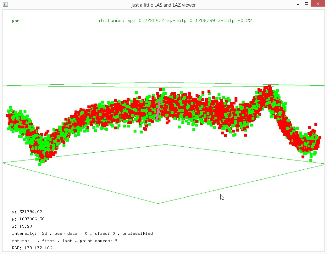
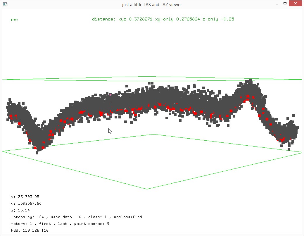
This produces 49 buffered tiles that will now be processed similarly to the workflow outlined for another lower-priced system that generates similarly „fluffy“ point clouds on hard surfaces, the Velodyne HLD-32E, described here and here. What do we mean with „fluffy“? We cut out a 1 meter slice across the road with the new ‚-keep_profile‘ filter and las2las and inspect it with lasview.

las2las ^
-i Samara\Livox\05_tiles_buffered\desman_331750_1093000.laz ^
-keep_profile 331790 1093071 331799 1093062 1 ^
-o slice.laz

lasview ^
-i slice.laz ^
-color_by_flightline ^
-kamera 0 274.922 43.7695 0.00195313 -0.0247396 1.94022 ^
-point_size 9

In the view below we pressed hot key twice ‚]‘ to exaggerate the z scale. The „fuzziness“ is that thickness of the point cloud in the middle of this flat tar road. It is around 20 to 25 centimeters and is equally evident in both flight lines. What is the correct ground surface through this 20 to 25 centimeter „thick“ road? We will compute a „mean ground“ that roughly falls into the middle of this „fluffy“ surface,

The next three lasthin runs mark a sub set of low candidate points for our lasground filtering. In every 25 cm by 25 cm, every 33 cm by 33 cm and every 50 cm by 50 cm area we reclassify the point closest to the 10th percentile as class 8. In the first call to lasthin we put all other points into class 1.

lasthin ^
-i Samara\Livox\05_tiles_buffered\desman_*.laz ^
-set_classification 1 ^
-step 0.25 -percentile 10 20 -classify_as 8 ^
-odir Samara\Livox\06_tiles_thinned_01 -olaz ^
-cores 4

lasthin ^
-i Samara\Livox\06_tiles_thinned_01\desman_*.laz ^
-step 0.3333 -percentile 10 20 -classify_as 8 ^
-odir Samara\Livox\06_tiles_thinned_02 -olaz ^
-cores 4

lasthin ^
-i Samara\Livox\06_tiles_thinned_02\desman_*.laz ^
-step 0.5 -percentile 10 20 -classify_as 8 ^
-odir Samara\Livox\06_tiles_thinned_03 -olaz ^
-cores 4

Below you can see the resulting points of the 10th percentile classified as class 8 in red.

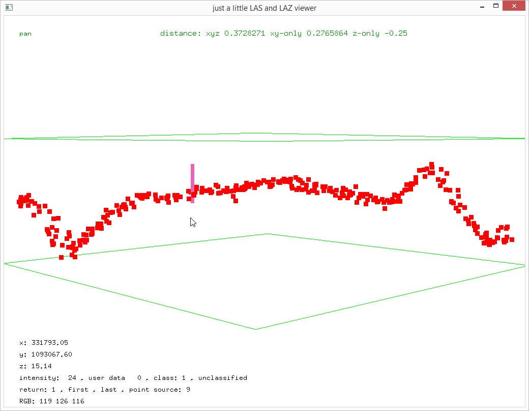
Operating only on the points classified as 8 (i.e. ignoring those classified as 1) we then run a ground classification with lasground using the following command line, which creates a „low ground“ classification. .

lasground ^
-i Samara\Livox\06_tiles_thinned_03\desman_*.laz ^
-ignore_class 1 ^
-town -ultra_fine ^
-ground_class 2 ^
-odir Samara\Livox\07_tiles_ground_low -olaz ^
-cores 4

Since this is an open road this classifies most of the red points as ground points.

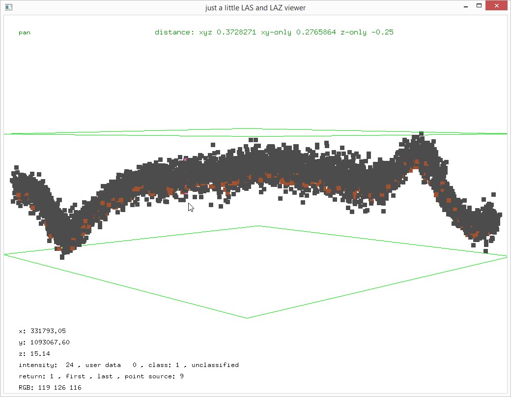
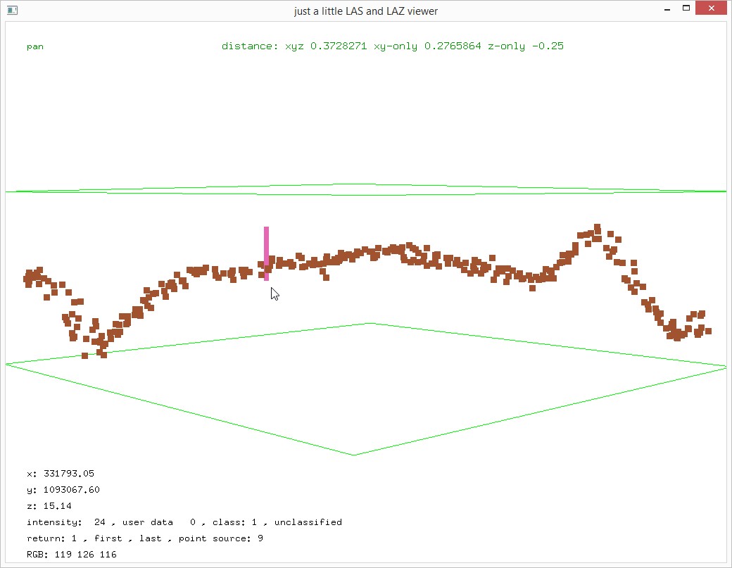
Using lasheight we then create a „thick ground“ by pulling all those points into the ground surface that are between 5 centimeter below and 17 centimeter above the „low ground“. For visualization purposes we temporarily use class 6 to capture this thickened ground.

lasheight ^
-i Samara\Livox\07_tiles_ground_low\desman_*.laz ^
-classify_between -0.05 0.17 6 ^
-odir Samara\Livox\07_tiles_ground_thick -olaz ^
-cores 4

The „thick ground“ is shown below in orange.

We go back to lasthin and reclassify in every 50 cm by 50 cm area the point closest to the 50th percentile as class 8. This is what we call the „median ground“.

lasthin ^
-i Samara\Livox\07_tiles_ground_thick\desman_*.laz ^
-ignore_class 1 ^
-step 0.5 -percentile 50 -classify_as 8 ^
-odir Samara\Livox\07_tiles_ground_median -olaz ^
-cores 4

The final „median ground“ points are shown in red below. These are the points we will use to eventually compute the DTM.

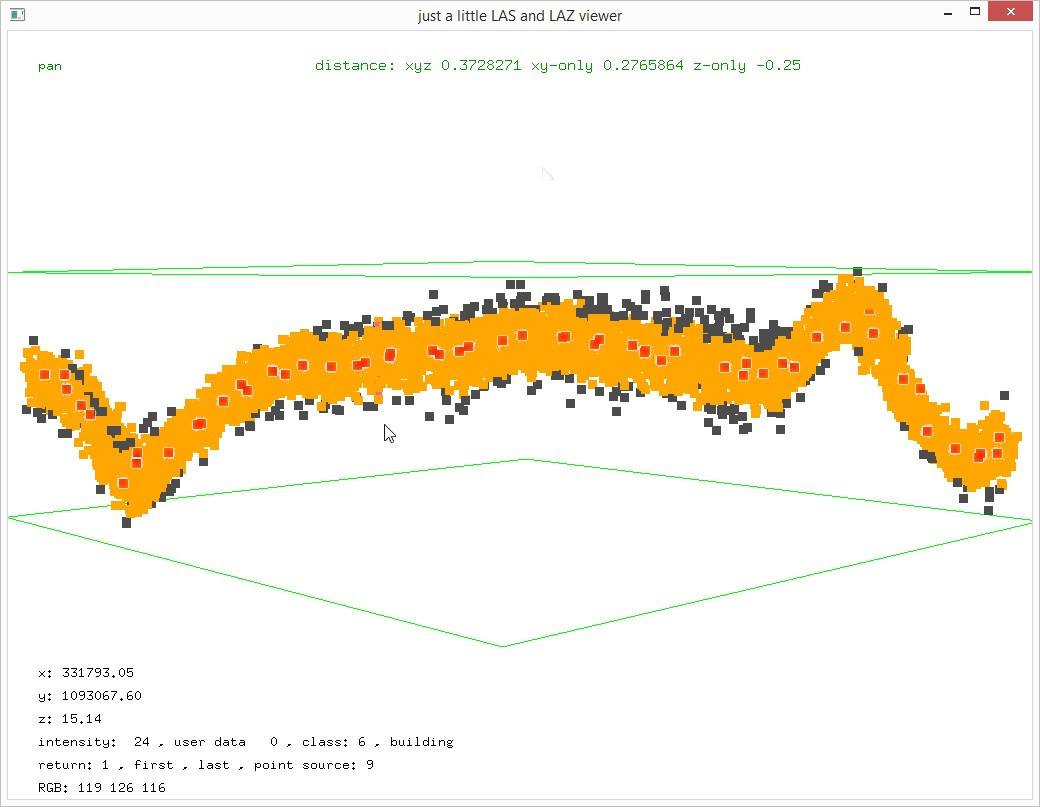
We complete the fully automated classification available in LAStools by running lasclassify with the following options. See the README file for what these options mean. Note that we move the „thick ground“ from the temporary class 6 to the proper class 2. The „median ground“ continues to be in class 8.

lasclassify ^
-i Samara\Livox\07_tiles_ground_median\desman_*.laz ^
-change_classification_from_to 6 2 ^
-rugged 0.3 -ground_offset 1.5 ^
-odir Samara\Livox\08_tiles_classified -olaz ^
-cores 4

Before the resulting tiles are published or shared with others we should remove the temporary buffers, which is done with lastile – the same tool that created the buffers.

lastile ^
-i Samara\Livox\08_tiles_classified\desman_*.laz ^
-remove_buffer ^
-odir Samara\Livox\09_tiles_final -olaz ^
-cores 4

And then we can publish the points via a Potree 3D Webportal using laspublish.

laspublish ^
-i Samara\Livox\09_tiles_final\desman_*.laz ^
-elevation ^
-title "Samara Mangroves" ^
-odir Samara\Livox\99_portal -o SamaraMangroves.html -olaz ^
-overwrite

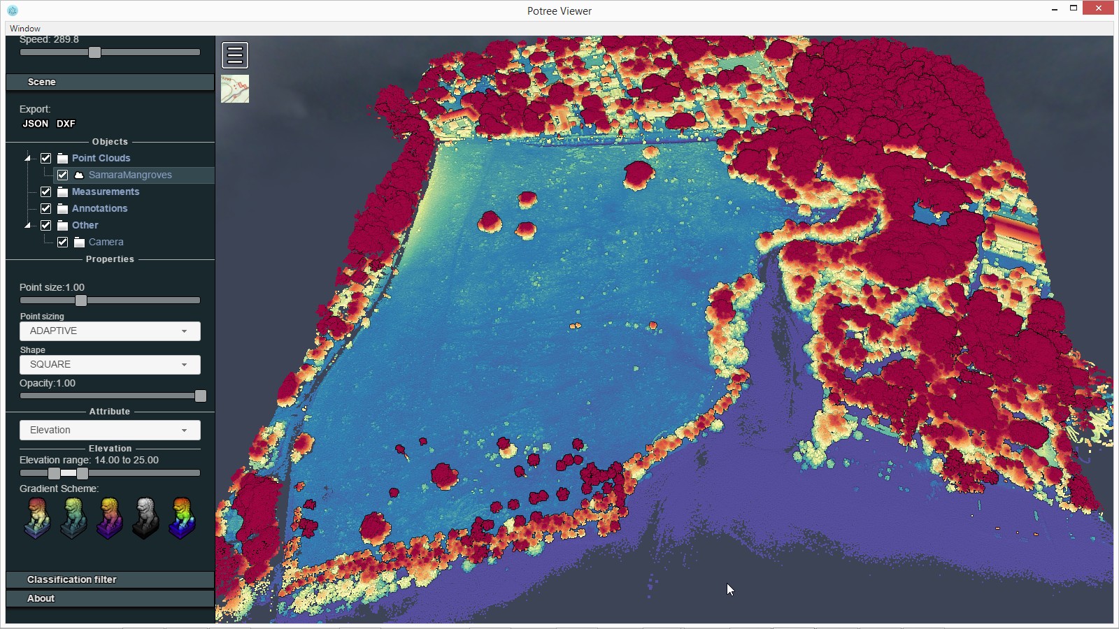
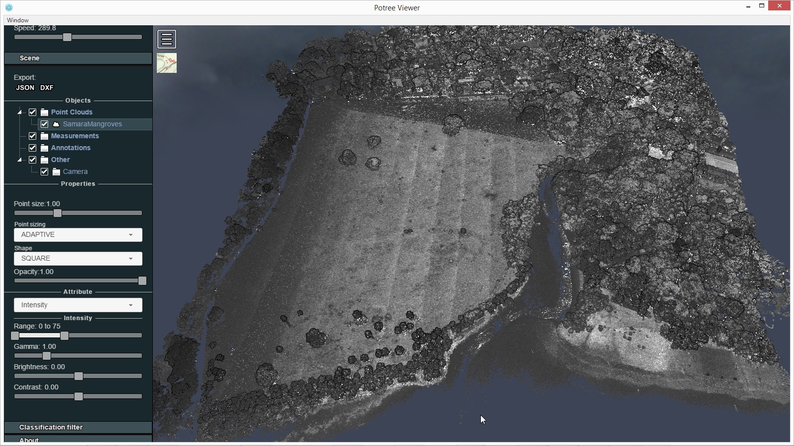
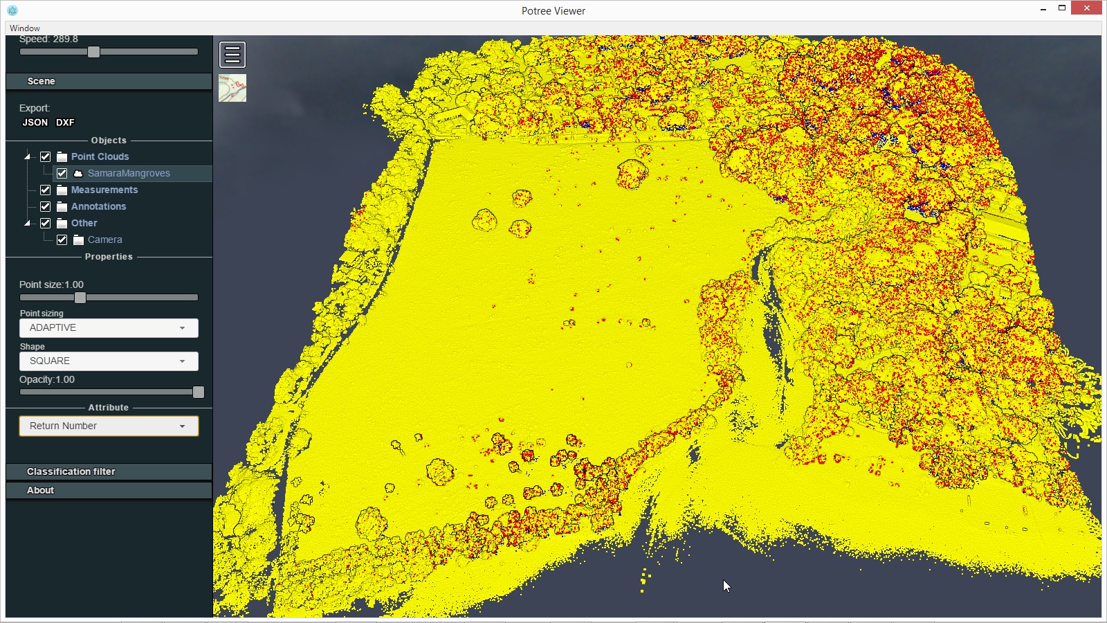
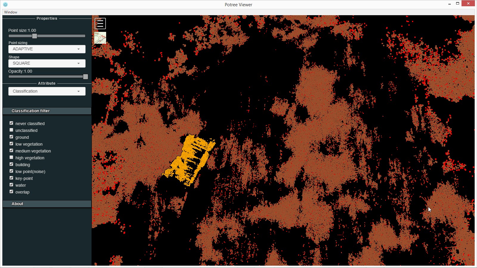
Below a screenshot of the resulting Potree 3D Web portal rendered with Potree Desktop. Inspecting the classification will reveal a number of errors that could be tweaked manually with lasview. How the point colors were generated is not described here but I used Google satellite imagery and mapped it with lascolor to the points. The elevation colors are mapped from 14 meters to 25 meters. The intensity image may help us understand why the black tar road on the left hand side that runs from the „Las Palmeras Condos“ to the beach in „Cangrejal“ has no samples. It seems the intensity is lower on this side which indicates that the drone may have flown higher here – too high to for the road to reflect enough photons. The yellow view of return type indicates that despite it’s multi-return capability, the Livox MID-40 LiDAR is mostly collecting single returns.

• 

• 

• 

• 

• 

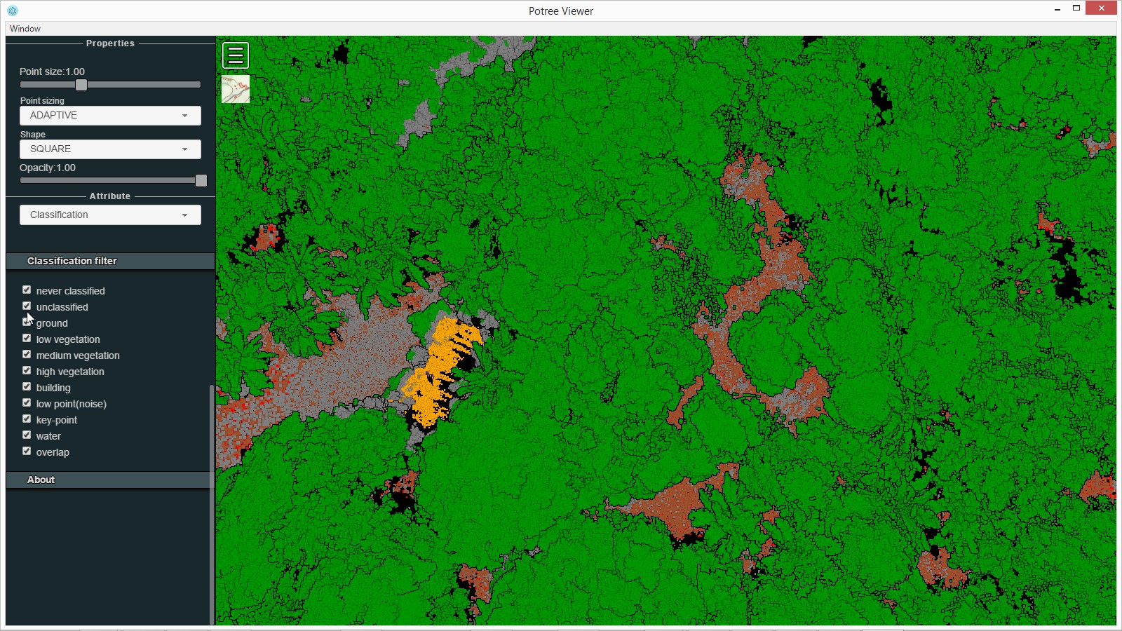
The penetration capability of the Livox MID-40 LiDAR was less good than we had hoped for. Below thick vegetation we have too few points on the ground to give us a good digital terrain model. In the visualization below you can see that below the dense vegetation there are large black areas which are completely void of points.

• 

• 

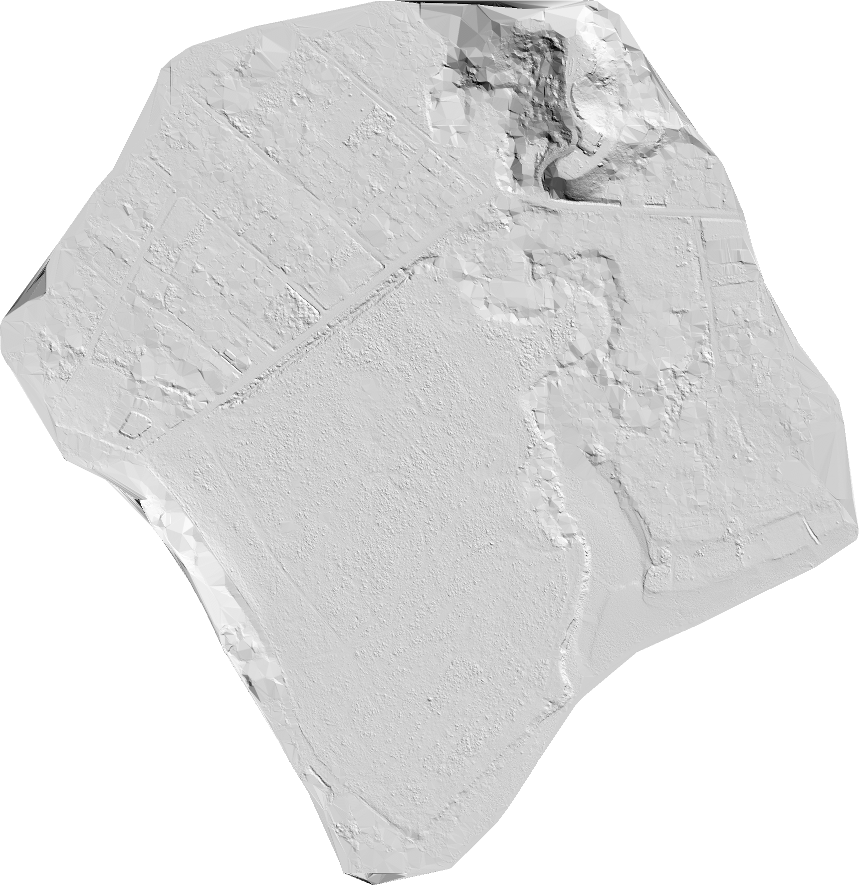
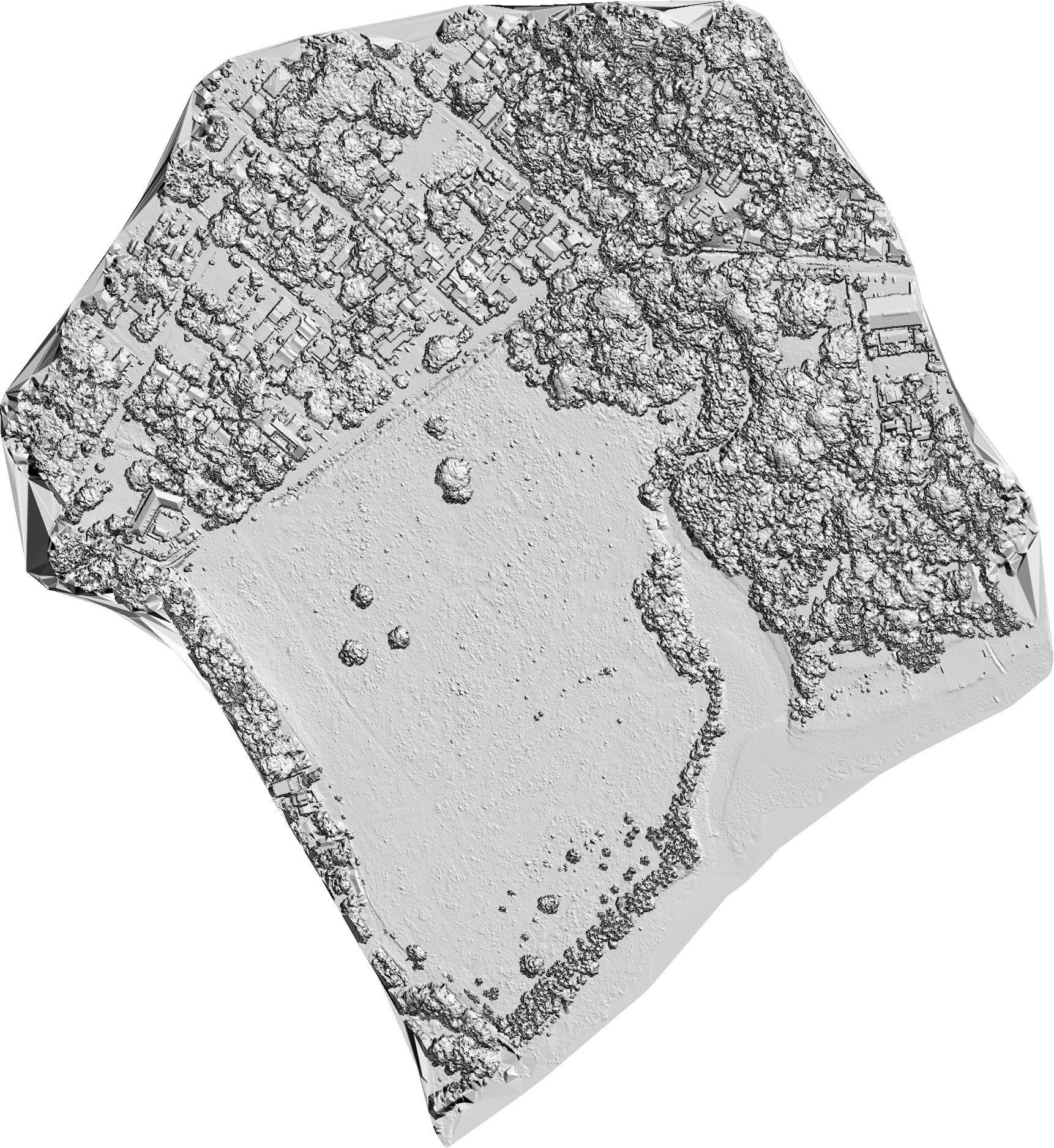
Now we produce the standard product DTM and DSM at a resolution of 50 cm. Because the total area is not that big we generate temporary tiles in „raster LAZ“ with las2dem and merge them into a single GeoTiff with blast2dem.

las2dem ^
-i Samara\Livox\07_tiles_ground_median\desman_*.laz ^
-keep_class 8 ^
-step 0.5 -use_tile_bb ^
-odir Samara\Livox\10_tiles_dtm_50cm -olaz ^
-cores 4

blast2dem ^
-i Samara\Livox\10_tiles_dtm_50cm*.laz -merged ^
-step 0.5 -hillshade ^
-o Samara\Livox\dtm_50cm.png

blast2dem ^
-i Samara\Livox\10_tiles_dtm_50cm*.laz -merged ^
-step 0.5 ^
-o Samara\Livox\dtm_50cm.tif

• 

• 

lasthin ^
-i Samara\Livox\07_tiles_ground_median\desman_*.laz ^
-step 0.5 -percentile 95 ^
-odir Samara\Livox\11_tiles_highest -olaz ^
-cores 4

las2dem ^
-i Samara\Livox\11_tiles_highest\desman_*.laz ^
-step 0.5 -use_tile_bb ^
-odir Samara\Livox\12_tiles_dsm_50cm -olaz ^
-cores 4

blast2dem ^
-i Samara\Livox\12_tiles_dsm_50cm*.laz -merged ^
-step 0.5 -hillshade ^
-o Samara\Livox\dsm_50cm.png

blast2dem ^
-i Samara\Livox\12_tiles_dsm_50cm*.laz -merged ^
-step 0.5 ^
-o Samara\Livox\dsm_50cm.tif

A big “Thank You!” to Nelson Mattie from LiDAR Latinoamerica for bringing his fancy drone to Samara and to Andre Jalobeanu from Bayesmap for his help in aligning the data. You can download the flight lines here and do the above processing on your own after downloading LAStools.