Points clouds from UAVs have become a common sight. Cheap consumer drones equipped with cameras produce points from images with increasing quality as photogrammetry software is improving. But vegetation is always a show stopper for point clouds generated from imagery data. Only an active sensing technique such as laser scanning can penetrate through the vegetation and generate points on the ground under the canopy of a forested area. Advances in UAV technology and the miniaturization of LiDAR systems have allowed lasers-scanning solutions for drones to enter the market.
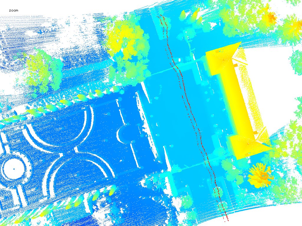
Last summer we attended the LiDAR for Drone 2017 Conference by YellowScan and processed some data sets flown with their Surveyor system that is built around the Velodyne VLP-16 Puck LiDAR scanner and the Applanix APX15 single board GNSS-Inertial solution. One common challenge observed in LiDAR data generated by the Velodyne Puck is that surfaces are not as „crisp“ as those generated by other laser scanners. Flat and open terrain surfaces are described by a layer of points with a „thickness“ of a few centimeter as you can see in the images below. This visualization uses a 10 meter by 5 meter cut-out of from this data set with the coordinate range [774280,774290) in x and [6279463,6279468) in y. Standard ground classification routines will „latch onto“ the lowermost envelope of these thick point layers and therefore produce a sub-optimal Digital Terrain Model (DTM).


In part this „thickness“ can be reduced by using fewer flightlines as the „thickness“ of each flightline by itself is lower but it is compounded when merging all flightlines together. However, deciding which (subset of) flightlines to use for which part of the scene to generate the best possible ground model is not an obvious tasks either and even per flightline there will be a remaining „thickness“ to deal with as can be seen in the following set of images.


In the following we show how to deal with „thickness“ in a layer of points describing a ground surface. We first produce a „lowest ground“ which we then widen into a „thick ground“ from which we then derive „median ground“ points that create a plausible terrain representation when interpolated by a Delaunay triangulation and rasterized onto a DTM. Step by step we process this example data set captured in a „live demo“ during the LiDAR for Drone 2017 Conference – the beautiful Château de Flaugergues in Montpellier, France where the event took place. You can download this data via this link if you would like to repeat these processing steps:
- six raw UAV flight strips above Flaugergues (261 MB)
Once you decompress the RAR file (e.g. with the UnRar.exe freeware) you will find six raw flight strips in LAS format and the trajectory of the UAV in ASCII text format as it was provided by YellowScan.
E:\LAStools\bin>dir Flaugergues
06/27/2017 08:03 PM 146,503,985 Flaugergues_test_demo_ppk_L1.las
06/27/2017 08:02 PM  91,503,103 Flaugergues_test_demo_ppk_L2.las
06/27/2017 08:03 PM 131,917,917 Flaugergues_test_demo_ppk_L3.las
06/27/2017 08:03 PM 219,736,585 Flaugergues_test_demo_ppk_L4.las
06/27/2017 08:02 PM 107,705,667 Flaugergues_test_demo_ppk_L5.las
06/27/2017 08:02 PM  74,373,053 Flaugergues_test_demo_ppk_L6.las
06/27/2017 08:03 PM   7,263,670 Flaugergues_test_demo_ppk_traj.txt
As usually we start with quality checking by visual inspection with lasview and by creating a textual report with lasinfo.
E:\LAStools\bin>lasview Flaugergues_test_demo_ppk_L1.las
E:\LAStools\bin>lasinfo Flaugergues_test_demo_ppk_L1.las
lasinfo (171011) report for Flaugergues_test_demo_ppk_L1.las
reporting all LAS header entries:
 file signature: 'LASF'
 file source ID: 1
 global_encoding: 1
 project ID GUID data 1-4: 00000000-0000-0000-0000-000000000000
 version major.minor: 1.2
 system identifier: 'YellowScan Surveyor'
 generating software: 'YellowReader by YellowScan'
 file creation day/year: 178/2017
 header size: 227
 offset to point data: 297
 number var. length records: 1
 point data format: 3
 point data record length: 34
 number of point records: 4308932
 number of points by return: 4142444 166488 0 0 0
 scale factor x y z: 0.001 0.001 0.001
 offset x y z: 774282 6279505 92
 min x y z: 774152.637 6279377.623 82.673
 max x y z: 774408.344 6279541.646 116.656
variable length header record 1 of 1:
 reserved 0
 user ID 'LASF_Projection'
 record ID 34735
 length after header 16
 description ''
 GeoKeyDirectoryTag version 1.1.0 number of keys 1
 key 3072 tiff_tag_location 0 count 1 value_offset 2154 - ProjectedCSTypeGeoKey: RGF93 / Lambert-93
reporting minimum and maximum for all LAS point record entries ...
 X -129363 126344
 Y -127377 36646
 Z -9327 24656
 intensity 0 65278
 return_number 1 2
 number_of_returns 1 2
 edge_of_flight_line 0 0
 scan_direction_flag 0 0
 classification 0 0
 scan_angle_rank -120 120
 user_data 75 105
 point_source_ID 1 1
 gps_time 219873.160527 219908.550379
 Color R 0 0
 G 0 0
 B 0 0
number of first returns: 4142444
number of intermediate returns: 0
number of last returns: 4142444
number of single returns: 3975956
overview over number of returns of given pulse: 3975956 332976 0 0 0 0 0
histogram of classification of points:
 4308932 never classified (0)
Nicely visible are the circular scanning patterns of the Velodyne VLP-16 Puck. We also notice that the trajectory of the UAV can be seen in the lasview visualization because the Puck was scanning the drone’s own landing gear. The lasinfo report tells us that point coordinates are stored with too much resolution (mm) and that points do not need to be stored using point type 3 (with RGB colors) because all RGB values are zero. We fix this with an initial run of las2las and also compress the raw strips to the LAZ format on 4 CPUs in parallel.
las2las -i Flaugergues\*.las ^
        -rescale 0.01 0.01 0.01 ^
        -auto_reoffset ^
        -set_point_type 1 ^
        -odir Flaugergues\strips_raw -olaz ^
        -cores 4
Next we do the usual check for flightline alignment with lasoverlap (README) which we consider to be by far the most important quality check. We compare the lowest elevation from different flightline per 25 cm by 25cm cell in all overlap areas. We consider a vertical difference of up to 5 cm as acceptable (color coded as white) and mark differences of over 30 cm (color coded as saturated red or blue).
lasoverlap -i Flaugergues\strips_raw\*.laz -faf ^
           -step 0.25 ^
           -min_diff 0.05 -max_diff 0.3 ^
           -odir Flaugergues\quality -o overlap.png


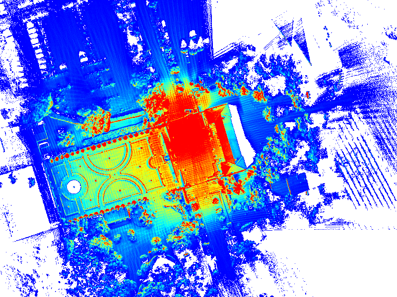
The vertical difference in open areas between the flightlines is slightly above 5 cm which we consider acceptable in this example. Depending on the application we recommend to investigate further where these differences come from and what consequences they may have for post processing. We also create a color-coded visualization of the last return density per 25 cm by 25 cm cell using lasgrid (README) with blue meaning less than 100 returns per square meter and red meaning more than 4000 returns per square meter.
lasgrid -i Flaugergues\strips_raw\*.laz -merged ^
        -keep_last ^
        -step 0.25 ^
        -point_density ^
        -false -set_min_max 100 4000 ^
        -odir Flaugergues\quality -o density_100_4000.png
As usual we start the LiDAR processing by reorganizing the flightlines into square tiles. Because of the variability in the density that is evident in the visualization above we use lastile (README) to create an adaptive tiling that starts with 200 m by 200 m tiles and then iterate to refine those tiles with over 10 million points down to smaller 25 m by 25 m tiles.
lastile -i Flaugergues\strips_raw\*.laz ^
        -apply_file_source_ID ^
        -tile_size 200 -buffer 8 -flag_as_withheld ^
        -refine_tiling 10000000 ^
        -odir Flaugergues\tiles_raw -o flauge.laz

lastile -i Flaugergues\tiles_raw\flauge*_200.laz ^
        -refine_tiles 10000000 ^
        -olaz ^
        -cores 4

lastile -i Flaugergues\tiles_raw\flauge*_100.laz ^
        -refine_tiles 10000000 ^
        -olaz ^
        -cores 4

lastile -i Flaugergues\tiles_raw\flauge*_50.laz ^
        -refine_tiles 10000000 ^
        -olaz ^
        -cores 4
Subsequent processing is faster when the points have a spatially coherent order. Therefore we rearrange the points into standard space-filling z-order using a call to lassort (README). We run this in parallel on as many cores as it makes sense (i.e. not using more cores than there are physical CPUs).
lassort -i Flaugergues\tiles_raw\flauge*.laz ^
        -odir Flaugergues\tiles_sorted -olaz ^
        -cores 4
Next we classify those points as noise that are isolated on a 3D grid of 1 meter cell size using lasnoise. See the README file of lasnoise for a description on the exact manner in which the isolated points are classified. We do this to eliminate low noise points that would otherwise cause trouble in the subsequent processing.
lasnoise -i Flaugergues\tiles_sorted\flauge*.laz ^
         -step 1 -isolated 5 ^
         -odir Flaugergues\tiles_denoised -olaz ^
         -cores 4
Next we mark the subset of lowest points on a 2D grid of 10 cm cell size with classification code 8 using lasthin (README) while ignoring the noise points with classification code 7 that were marked as noise in the previous step.
lasthin -i Flaugergues\tiles_denoised\flauge*.laz ^
        -ignore_class 7 ^
        -step 0.1 -lowest ^
        -classify_as 8 ^
        -odir Flaugergues\tiles_lowest -olaz ^
        -cores 4
Considering only the resulting points marked with classification 8 we then create a temporary ground classification that we refer to as the „lowest ground“. For this we run lasground (README) with a set of suitable parameters that were found by experimentation on two of the most complex tiles from the center of the survey.
lasground -i Flaugergues\tiles_lowest\flauge*.laz ^
          -ignore_class 0 7 ^
          -step 5 -hyper_fine -bulge 1.5 -spike 0.5 ^
          -odir Flaugergues\tiles_lowest_ground -olaz ^
          -cores 4
We then „thicken“ this „lowest ground“ by classifying all points that are between 2 cm below and 15 cm above the lowest ground to a temporary classification code 6 using the lasheight (README) tool. Depending on the spread of points in your data set you may want to tighten this range accordingly, for example when processing the flightlines acquired by the Velodyne Puck individually. We picked our range based on the visual experiments with „drop lines“ and „rise lines“ in the lasview viewer that are shown in images above.
lasheight -i Flaugergues\tiles_lowest_ground\flauge*.laz ^
          -do_not_store_in_user_data ^
          -classify_between -0.02 0.15 6 ^
          -odir Flaugergues\tiles_thick_ground -olaz ^
          -cores 4


The final ground classification is obtained by creating the „median ground“ from the „thick ground“. This uses a brand-new option in the lasthin (README) tool of LAStools. The new ‚-percentile 50 10‘ option selects the point that is closest to the specified percentile of 50 of all point elevations within a grid cell of a specified size given there are at least 10 points in that cell. The selected point either survives the thinning operation or gets marked with a specified classification code or flag.
lasthin -i Flaugergues\tiles_thick_ground\flauge*.laz ^
        -ignore_class 0 1 7 ^
        -step 0.1 -percentile 50 10 ^
        -classify_as 8 ^
        -odir Flaugergues\tiles_median_ground_10_10cm -olaz ^
        -cores 4

lasthin -i Flaugergues\tiles_median_ground_10_10cm\%NAME%*.laz ^
        -ignore_class 0 1 7 ^
        -step 0.2 -percentile 50 10 ^
        -classify_as 8 ^
        -odir Flaugergues\tiles_median_ground_10_20cm -olaz ^
        -cores 4

lasthin -i Flaugergues\tiles_median_ground_10_20cm\%NAME%*.laz ^
        -ignore_class 0 1 7 ^
        -step 0.4 -percentile 50 10 ^
        -classify_as 8 ^
        -odir Flaugergues\tiles_median_ground_10_40cm -olaz ^
        -cores 4

lasthin -i Flaugergues\tiles_median_ground_10_40cm\flauge*.laz ^
        -ignore_class 0 1 7 ^
        -step 0.8 -percentile 50 10 ^
        -classify_as 8 ^
        -odir Flaugergues\tiles_median_ground_10_80cm -olaz ^
         -cores 4
We now compare a triangulation of the median ground points with a triangulation of the highest and the lowest points per 10 cm by 10 cm cell to demonstrate that – at least in open areas – we really have computed a median ground surface.


Finally we raster the tiles with the las2dem (README) tool onto binary elevation grids in BIL format. Here we make the resolution dependent on the tile size, giving the 25 meter and 50 meter tiles the highest resolution of 10 cm and rasterize the 100 meter and 200 meter tiles at 20 cm and 40 cm respectively.
las2dem -i Flaugergues\tiles_median_ground_10_80cm\*_25.laz ^
        -i Flaugergues\tiles_median_ground_10_80cm\*_50.laz ^
        -keep_class 8 ^
        -step 0.1 -use_tile_bb ^
        -odir Flaugergues\tiles_dtm -obil ^
        -cores 4

las2dem -i Flaugergues\tiles_median_ground_10_80cm\*_100.laz ^
        -keep_class 8 ^
        -step 0.2 -use_tile_bb ^
        -odir Flaugergues\tiles_dtm -obil ^
        -cores 4

las2dem -i Flaugergues\tiles_median_ground_10_80cm\*_200.laz ^
        -keep_class 8 ^
        -step 0.4 -use_tile_bb ^
        -odir Flaugergues\tiles_dtm -obil ^
        -cores 4
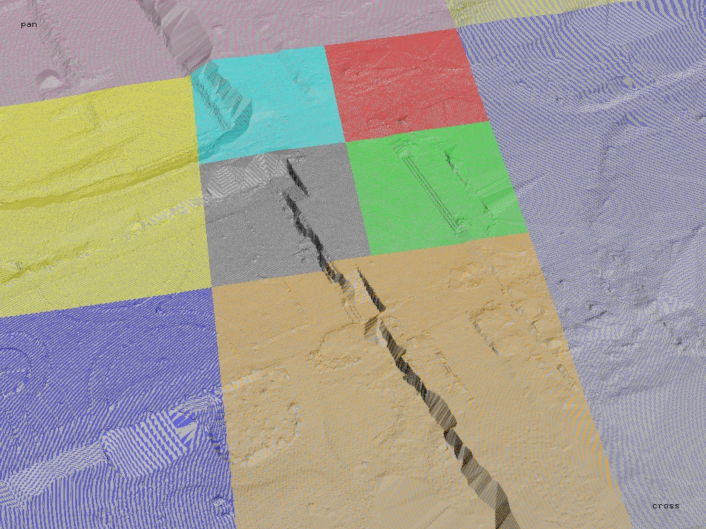
Because all LAStools can read BIL files via on the fly conversion from rasters to points we can visually inspect the resulting elevation rasters with the lasview (README) tool. By adding the ‚-faf‘ or ‚files_are_flightlines‘ argument we treat the BIL files as if they were different flightlines which allows us to assign different color to points from different files to better inspect the transitions between tiles. The ‚-points 10000000‘ argument instructs lasview to load up to 10 million points into memory instead of the default 5 million.
lasview -i Flaugergues\tiles_dtm\*.bil -faf ^
        -points 10000000
For visual comparison we also produce a DSM and create hillshades. Note that the workflow for DSM creation shown below produces a „highest DSM“ that will always be a few centimeter above the „median DTM“. This will be noticeable only in open areas of the terrain where the DSM and the DTM should coincide and their elevation should be identical.


lasthin -i Flaugergues\tiles_denoised\flauge*.laz ^
        -keep_z_above 110 ^
        -filtered_transform ^
        -set_classification 18 ^
        -ignore_class 7 18 ^
        -step 0.1 -highest ^
        -classify_as 5 ^
        -odir Flaugergues\tiles_highest -olaz ^
        -cores 4

las2dem -i Flaugergues\tiles_highest\*_25.laz ^
        -i Flaugergues\tiles_highest\*_50.laz ^
        -keep_class 5 ^
        -step 0.1 -use_tile_bb ^
        -odir Flaugergues\tiles_dsm -obil ^
        -cores 4

las2dem -i Flaugergues\tiles_highest\*_100.laz ^
        -keep_class 5 ^
        -step 0.2 -use_tile_bb ^
        -odir Flaugergues\tiles_dsm -obil ^
        -cores 4

las2dem -i Flaugergues\tiles_highest\*_200.laz ^
        -keep_class 5 ^
        -step 0.4 -use_tile_bb ^
        -odir Flaugergues\tiles_dsm -obil ^
        -cores 4
We thank YellowScan for challenging us to process their drone LiDAR with LAStools in order to present results at their LiDAR for Drone 2017 Conference and for sharing several example data sets with us, including the one used here.
One potential use of low altitude below the cloud UAV LiDAR payload is for agricultural land assessment how arable they are (meaning how good as it for agricultural use). The slope of the landscape and where it faces relative to the sun is one important criteria for good land, This article shows that the derived DTM may not be that fine since the scanning technology is not the usual linear laser scanning system used. That could be a potential problem since soil is also tilled on each beginning cycle of planting also common planted crops may not even reach more than 2 meters even at their maturity (fruit bearing tress do of course). Question now is what could be a suitable LiDAR scanning technology that can work for agriculture that could still fit and light enough to be carried by a UAV Multirotor.
Pingback: First Look with LAStools at LiDAR from Hovermap Drone by CSIRO | rapidlasso GmbH
Pingback: New Step-by-Step Tutorial for Velodyne Drone LiDAR with Snoopy from LidarUSA | rapidlasso GmbH