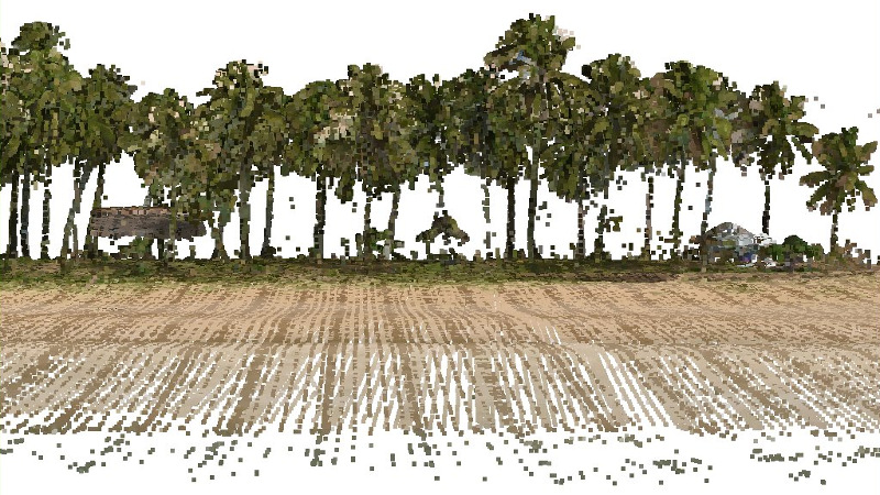
In this tutorial we are removing some „tricky“ low noise from LiDAR point clouds in order to produce a high-resolution Digital Terrain Model (DTM). The data was flown above a tropical beach and mangrove area in the Philippines using a VUX-1 UAV based system from RIEGL mounted on a helicopter. The survey was done as a test flight by AB Surveying who have the capacity to fly such missions in the Philippines and who have allowed us to share this data with you for educational purposes. You can download the data (1 GB) here. It covers a popular twin beach knows as „Nacpan“ near El Nido in Palawan (that we happen to have visited in 2014).
We start our usual quality check with a run of lasinfo. We add the ‚-cd‘ switch to compute an average point density and the ‚-histo gps_time 1‘ switch to produce a 1 second histogram for the GPS time stamps.
lasinfo -i lalutaya.laz ^
        -cd ^
        -histo gps_time 1 ^
        -odix _info -otxt
You can download the resulting lasinfo report here. It tells us that there are 118,740,310 points of type 3 (with RGB colors) with an average density of 57 last returns per square meter. The point coordinates are in the „PRS92 / Philippines 1“ projection with EPSG code 3121 that is based on the „Clarke 1866“ ellipsoid.
Datum Transform
We prefer to work in an UTM projection based on the „WGS 1984“ ellipsoid, so we will first perform a datum transform based on the seven parameter Helmert transformation – a capacity that was recently added to LAStools. For this we first need a transform to get to geocentric or Earth-Centered Earth-Fixed (ECEF) coordinates on the current „Clarke 1866“ ellipsoid, then we apply the Helmert transformation that operates on geocentric coordinates and whose parameters are listed in the TOWGS84 string of EPSG code 3121 to get to geocentric or ECEF coordinates on the „WGS 1984“ ellipsoid. Finally we can convert the coordinates to the respective UTM zone. These three calls to las2las accomplish this.
las2las -i lalutaya.laz ^
        -remove_all_vlrs ^
        -epsg 3121 ^
        -target_ecef ^
        -odix _ecef_clark1866 -olaz

las2las -i lalutaya_ecef_clark1866.laz ^
        -transform_helmert -127.62,-67.24,-47.04,-3.068,4.903,1.578,-1.06 ^
        -wgs84 -ecef ^
        -ocut 10 -odix _wgs84 -olaz

las2las -i lalutaya_ecef_wgs84.laz ^
        -target_utm auto ^
        -ocut 11 -odix _utm -olaz
In these steps we implicitly reduced the resolution that each coordinate was stored with from quarter-millimeters (i.e. scale factors of 0.00025) to the default of centimeters (i.e. scale factors of 0.01) which should be sufficient for subsequent vegetation analysis. The LAZ files also compress better when coordinates a lower resolution so that the ‚lalutaya_utm.laz‘ file is over 200 MB smaller than the original ‚lalutaya.laz‘ file. The quantization error this introduces is probably still below the overall scanning error of this helicopter survey.
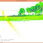
Flightline Recovery
Playing back the file visually with lasview suggests that it contains more than one flightline. Unfortunately the point source ID field of the file is not properly populated with flightline information. However, when scrutinizing the GPS time stamp histogram in the lasinfo report we can see an occasional gap. We highlight two of these gaps in red between GPS second 540226 and 540272 and GPS second 540497 and 540556 in this excerpt from the lasinfo report:
gps_time histogram with bin size 1
[...]
 bin 540224 has 125768
 bin 540225 has 116372
 bin 540226 has 2707
 bin 540272 has 159429
 bin 540273 has 272049
 bin 540274 has 280237
[...]
 bin 540495 has 187103
 bin 540496 has 180421
 bin 540497 has 126835
 bin 540556 has 228503
 bin 540557 has 275025
 bin 540558 has 273861
[...]
We can use lasplit to recover the original flightlines based on gaps in the continuity of GPS time stamps that are bigger than 10 seconds:
lassplit -i lalutaya_utm.laz ^
         -recover_flightlines_interval 10 ^
         -odir strips_raw -o lalutaya.laz
This operation splits the points into 11 separate flightlines. The points within each flightline are stored in the order that the vendor software – which was RiPROCESS 1.7.2 from RIEGL according to the lasinfo report – had written them to file. We can use lassort to bring them back into the order they were acquired in by sorting first on the GPS time stamp and then on the return number field:
lassort -i strips_raw\*.laz ^
        -gps_time -return_number ^
        -odir strips_sorted -olaz ^
        -cores 4
Now we turn the sorted flightlines into tiles (with buffers !!!) for further processing. We also erase the current classification of the data into ground (2) and medium vegetation (4) as a quick visual inspection with lasview immediately shows that those are not correct:
lastile -i strips_sorted\*.laz ^
        -files_are_flightlines ^
        -set_classification 0 ^
        -tile_size 250 -buffer 30 -flag_as_withheld ^
        -odir tiles_raw -o lalu.laz
Quality Checking
Next comes the standard check of flightline overlap and alignment check with lasoverlap. Once more it become clear why it is so important to have flightline information. Without we may have missed what we are about to notice. We create false color images load into Google Earth to visually assess the situation. We map all absolute differences between flightlines below 5 cm to white and all absolute differences above 30 cm to saturated red (positive) or blue (negative) with a gradual shading from white to red or blue for any differences in between. We also create an overview KML file that lets us quickly see in which tile we can find the points for a particular area of interest with lasboundary.
lasoverlap -i tiles_raw\*.laz ^
           -step 1 -min_diff 0.05 -max_diff 0.30 ^
           -odir quality -opng ^
           -cores 4

lasboundary -i tiles_raw\*.laz ^
            -use_tile_bb -overview -labels ^
            -o quality\overview.kml
The resulting visualizations show (a) that our datum transform to the WGS84 ellipsoid worked because the imagery aligns nicely with Google Earth and (b) that there are several issues in the data that require further scrutiny.


In general the data seems well aligned (most open areas are white) but there are blue and red lines crossing the survey area. With lasview have a closer look at the visible blue lines running along the beach in tile ‚lalu_765000_1252750.laz‘ by repeatedly pressing ‚x‘ to select a different subset and ‚x‘ again to view this subset up close while pressing ‚c‘ to color it differently:
lasview -i tiles_raw\lalu_765000_1252750.laz
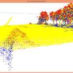

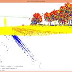

These lines of erroneous points do not only happen along the beach but also in the middle of and below the vegetation as can be seen below:


Our initial hope was to use the higher than usual intensity of these erroneous points to reclassify them to some classification code that we would them exclude from further processing. Visually we found that a reasonable cut-off value for this tile would be an intensity above 35000:
lasview -i tiles_raw\lalu_765000_1252750.laz ^
        -keep_intensity_above 35000 ^
        -filtered_transform ^
        -set_classification 23


However, while this method seems successful on the tile shown above it fails miserably on others such as ‚lalu_764250_1251500.laz‘ where large parts of the beach are very reflective and result in high intensity returns to to the dry white sand:
lasview -i tiles_raw\lalu_764250_1251500.laz ^
        -keep_intensity_above 35000 ^
        -filtered_transform ^
        -set_classification 23


Low Noise Removal
In the following we describe a workflow that can remove the erroneous points below the ground so that we can at least construct a high-quality DTM from the data. This will not, however, remove the erroneous points above the ground so a subsequent vegetation analysis would still be affected. Our approach is based on two obervations (a) the erroneous points affect only a relatively small area and (b) different flightlines have their erroneous points in different areas. The idea is to compute a set of coarser ground points separately for each flightline and – when combining them in the end – to pick higher ground points over lower ones. The combined points should then define a surface that is above the erroneous below-ground points so that we can mark them with lasheight as not to be used for the actual ground classification done thereafter.
The new huge_las_file_extract_ground_points_only.bat example batch script that you can download here does all the work needed to compute a set of coarser ground points for each flightline. Simply edit the file such that the LAStools variable points to your LAStools\bin folder and rename it to end with the *.bat extension. Then run:
huge_las_file_extract_ground_points_only strips_sorted\lalutaya_0000001.laz strips_ground_only\lalutaya_0000001.laz
huge_las_file_extract_ground_points_only strips_sorted\lalutaya_0000002.laz strips_ground_only\lalutaya_0000001.laz
huge_las_file_extract_ground_points_only strips_sorted\lalutaya_0000003.laz strips_ground_only\lalutaya_0000001.laz
...
huge_las_file_extract_ground_points_only strips_sorted\lalutaya_0000009.laz strips_ground_only\lalutaya_0000009.laz
huge_las_file_extract_ground_points_only strips_sorted\lalutaya_0000010.laz strips_ground_only\lalutaya_0000010.laz
huge_las_file_extract_ground_points_only strips_sorted\lalutaya_0000011.laz strips_ground_only\lalutaya_0000011.laz
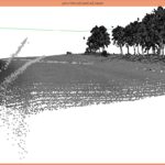
The details on how this batch script works – a pretty standard tile-based multi-core processing workflow – are given as comments in this batch script. Now we have a set of individual ground points computed separately for each flightline and some will include erroneous points below the ground that the lasground algorithm by its very nature is likely to latch on to as you can see here:


The trick is now to utilize the redundancy of multiple scans per area and – when combining flightlines – to pick higher rather than lower ground points in overlap areas by using the ground point closest to the 75th elevation percentile per 2 meter by 2 meter area with at least 3 or more points with lasthin:
lasthin -i strips_ground_only\*.laz -merged ^
        -step 2 -percentile 75 3 ^
        -o lalutaya_ground_only_2m_75_3.laz
There are still some non-ground points in the result as ground-classifying of flightlines individually often results in vegetation returns being included in sparse areas along the edges of the flight lines but we can easily get rid of those:
lasground_new -i lalutaya__ground_only_2m_75_3.laz ^
              -town -hyper_fine ^
              -odix _g -olaz
We sort the remaining ground points into a space-filling curve order with lassort and spatially index them with lasindex so they can be efficiently accessed by lasheight in the next step.
lassort -i lalutaya__ground_only_2m_75_3_g.laz ^
        -keep_class 2 ^
        -o lalutaya_ground.laz

lasindex -i lalutaya_ground.laz
Finally we have the means to robustly remove the erroneous points below the ground from all tiles. We use lasheight with the ground points we’ve just so painstakingly computed to classify all points 20 cm or more below the ground surface they define into classification code 23. Later we simply can ignore this classification code during processing:
lasheight -i tiles_raw\*.laz ^
          -ground_points lalutaya_ground.laz ^
          -do_not_store_in_user_data ^
          -classify_below -0.2 23 ^
          -odir tiles_cleaned -olaz ^
          -cores 4


Rather than trying to ground classify all remaining points we run lasground on a thinned subset of all points. For this we mark the lowest point in every 20 cm by 20 cm grid cell with some temporary classification code such as 6.
lasthin -i tiles_cleaned\*.laz ^
        -ignore_class 23 ^
        -step 0.20 -lowest -classify_as 6 ^
        -odir tiles_thinned -olaz ^
        -cores 4
Finally we can run lasground to compute the ground classification considering all points with classification code 6 by ignoring all points with classification codes 23 and 0.
lasground_new -i tiles_thinned\*.laz ^
              -ignore_class 23 0 ^
              -city -hyper_fine ^
              -odir tiles_ground_new -olaz ^
              -cores 4
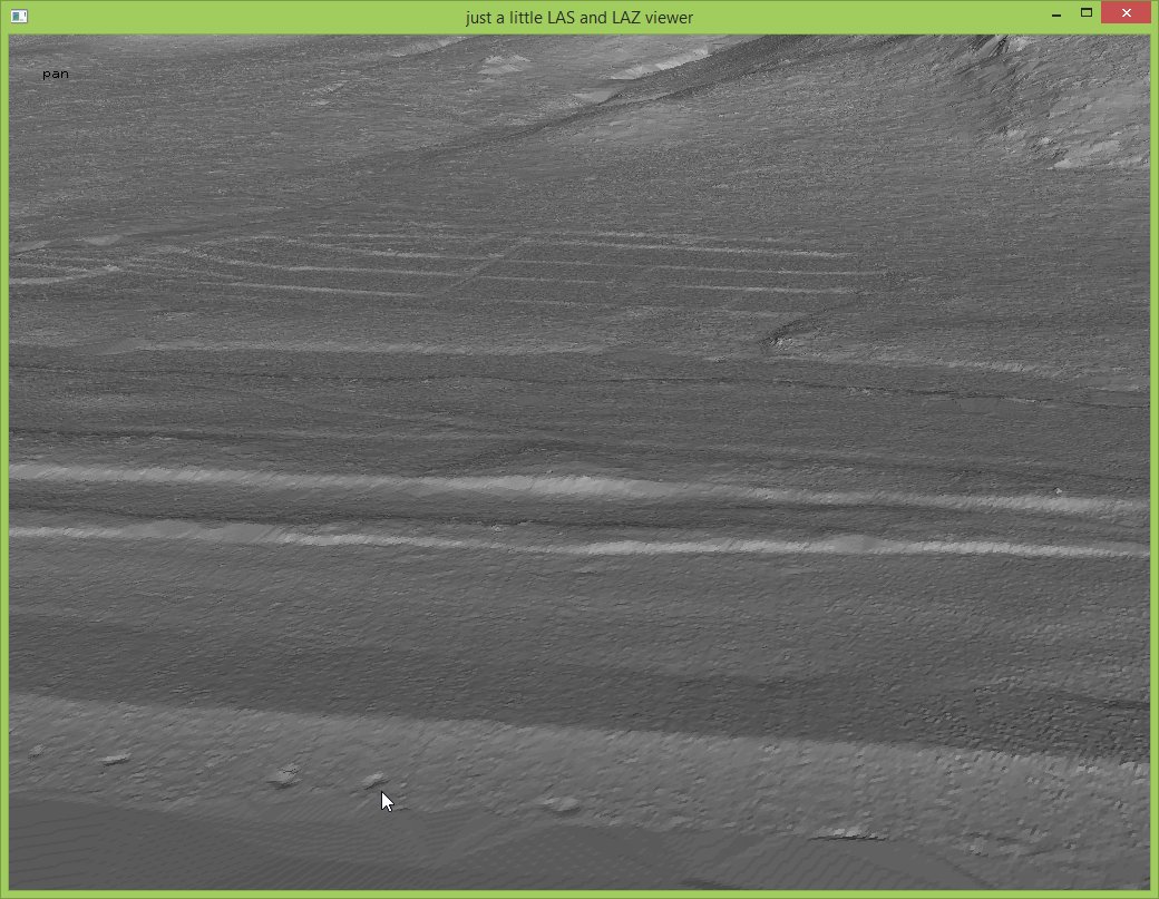
And finally we can create a DTM with a resolution of 25 cm using las2dem and the result is truly beautiful:
las2dem -i tiles_ground_new\*.laz ^
        -keep_class 2 ^
        -step 0.25 -use_tile_bb ^
        -odir tiles_dtm_25cm -obil ^
        -cores 4
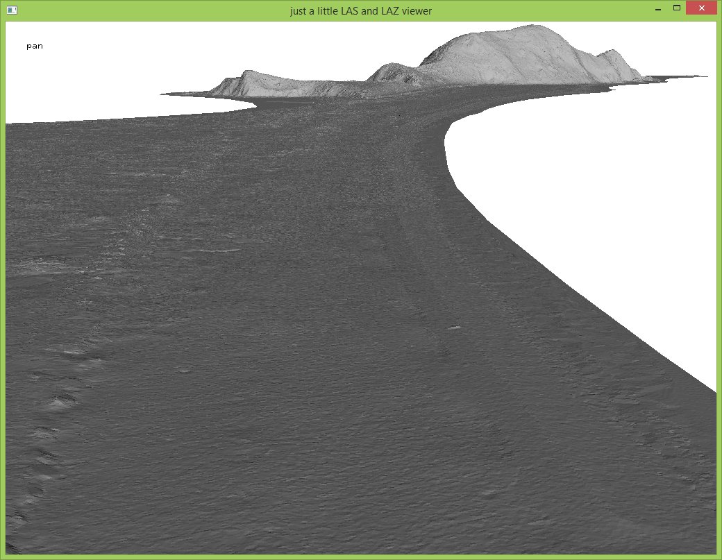
We have to admit that a few bumps are left (see mouse cursor below) but adjusting the parameters presented here is left as an exercise to the reader.
We would again like to acknowledge AB Surveying whose generosity has made this blog article possible. They have the capacity to fly such missions in the Philippines and who have allowed us to share this data with you for educational purposes.
What is the reason for this noise? At first I hypothesized – without further explanation – that this may have to do with the waveform processing. That may not be an entirely accurate description. In a discussion with another LAStools user who has flown the RIEGL VUX-1 UAV sensor we concluded that the noise we are removing here was to a large degree caused by either flying outside the set MTA-zone (in terms of range) or by processing the data in the wrong MTA-zone (which is nearly the same). One could potentially confirm this by having the flight trajectory. It would also be good to know what pulse rate the survey was flown with.
Being outside of the assumed MTA-zone happens easily with the VUX. This is according to the user that I have discussed this with who has done that himself on occasion. However, one can eliminate the wrong returns – in case they are indeed caused by a wrong MTA-zone – quite easily if one still has access to the original SDF files and the RIEGL processing software.
That said … the „free data“ we obtained from AB Surveying were just the „test output“ from a „test flight“ for a new system that had been recently acquired, hence such issues are to be expected.