First Look with LAStools at LiDAR from Hovermap Drone by CSIRO

Last December we had a chance to visit the team of Dr. Stefan Hrabar at CSIRO in Pullenvale near Brisbane who work on a drone LiDAR system called Hovermap. This SLAM-based system is mainly developed for the purpose of autonomous flight and exploration of GPS-denied environments such as buildings, mines and tunnels. But as the SLAM algorithm continuously self-registers the scan lines it produces a LiDAR point cloud that in itself is a nice product. We started our visit with a short test flight around the on-site tower. You can download the LiDAR data and the drone trajectory of this little survey here:

• the LiDAR data
• the drone trajectory

The Hovermap system is based on the Velodyne Puck Lite (VLP-16) that is much cheaper and more light-weight than many other LiDAR systems. One interesting tidbit in the Hovermap setup is that the scanner is installed such that the entire Puck is constantly rotating as you can see in this video. But  the Velodyne Puck is also known to produce somewhat „fluffy“ surfaces with a thickness of a few centimeters. In a previous blog post with data from the YellowScan Surveyor system (that is also based on the Puck) we used a „median ground“ surface to deal with the „fluff“. In the following we will have a look at the LiDAR data produced by Hovermap and how to process it with LAStools.

As always we start with a lasinfo report that computes the average density ‚-cd‘ and histograms for the intensity and the GPS time:

lasinfo -i CSIRO_Tower\results.laz ^
        -cd ^
        -histo intensity 16 -histo gps_time 2 ^
        -odir CSIRO_Tower\quality -odix _info -otxt

A few excerpts of the resulting lasinfo report that you can download here are below:

lasinfo (180409) report for 'CSIRO_Tower\results.laz'
[...]
 number of point records: 16668904
 number of points by return: 0 0 0 0 0
 scale factor x y z: 0.0001 0.0001 0.0001
 offset x y z: -5.919576153930379 22.785394470724583 9.535698734939086
 min x y z: -138.6437 -125.2552 -34.1510
 max x y z: 126.8046 170.8260 53.2224
WARNING: full resolution of min_x not compatible with x_offset and x_scale_factor: -138.64370561381907
WARNING: full resolution of min_y not compatible with y_offset and y_scale_factor: -125.25518631070418
WARNING: full resolution of min_z not compatible with z_offset and z_scale_factor: -34.150966206894068
WARNING: full resolution of max_x not compatible with x_offset and x_scale_factor: 126.80455330595831
WARNING: full resolution of max_y not compatible with y_offset and y_scale_factor: 170.82597525215334
WARNING: full resolution of max_z not compatible with z_offset and z_scale_factor: -34.150966206894068
[...]
 gps_time 121.288045 302.983110
WARNING: 2 points outside of header bounding box
[...]
covered area in square units/kilounits: 51576/0.05
point density: all returns 323.19 last only 318.40 (per square units)
 spacing: all returns 0.06 last only 0.06 (in units)
WARNING: for return 1 real number of points by return is 16424496 but header entry was not set.
WARNING: for return 2 real number of points by return is 244408 but header entry was not set.
[...]
real max z larger than header max z by 0.000035
real min z smaller than header min z by 0.000035
[...]

Most of these warnings have to do with poorly chosen offset values in the LAS header that have many decimal digits instead of being nice round numbers. The points are stored with sub-millimeter resolution (scale factors of 0.0001) which is unnecessarily precise for a UAV flying a Velodyne Puck where the overall system error can be expected to be on the order of a few centimeters. Also the histogram of return numbers in the LAS header was not populated. We can fix these issues with one call to las2las:

las2las -i CSIRO_Tower\results.laz ^
        -rescale 0.01 0.01 0.01 ^
        -auto_reoffset ^
        -odix _fixed -olaz

If you create another lasinfo report on the fixed file you will see that all the warnings have gone. The file size is now also only 102 MB instead of 142 MB because centimeter coordinate compress much better than sub-millimeter coordinates.

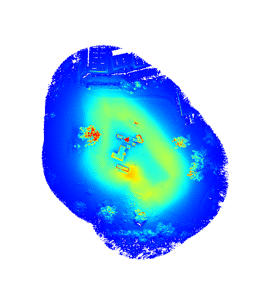
The average density of 318 last return per square meter reported by lasinfo is not that useful for a UAV survey because it does account for the highly varying distribution of LiDAR returns in the area surveyed. With lasgrid we can get a much more clear picture of that.

lasgrid -i CSIRO_Tower\results_fixed.laz ^
        -last_only ^
        -step 0.5 -use_bb -density ^
        -false -set_min_max 0 1500 ^
        -o CSIRO_Tower\quality\density_0_1500.png

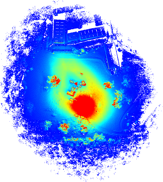
The red dot in the point density indicated an area with over 1500 last returns per square meter. No surprise that this is the take-off and touch-down location of the copter drone. Naturally this spot is completely over-scanned compared to the rest of the area. We can remove these points with the help of the timestamps by cutting off the start and the end of the recording.

The total recording time including take-off, flight around the tower, and touch-down was around 180 seconds or 3 minutes as the lasinfo report tells us. Note that the recorded time stamps are neither „GPS Week Time“ nor „Adjusted Standard GPS Time“ but an internal system time. By visualizing the trajectory of the UAV with lasview while binning the timestamps into the intensity field we can easily determine what interval of timestamps describes the actual survey flight. First we convert the drone trajectory from the textual ASCII format to the LAZ format with txt2las:

txt2las -i CSIRO_Tower\results_traj.txt ^
        -skip 1 ^
        -parse txyz ^
        -set_classification 12 ^
        -olaz

lasview -i CSIRO_Tower\results_traj.laz ^
        -bin_gps_time_into_intensity 1

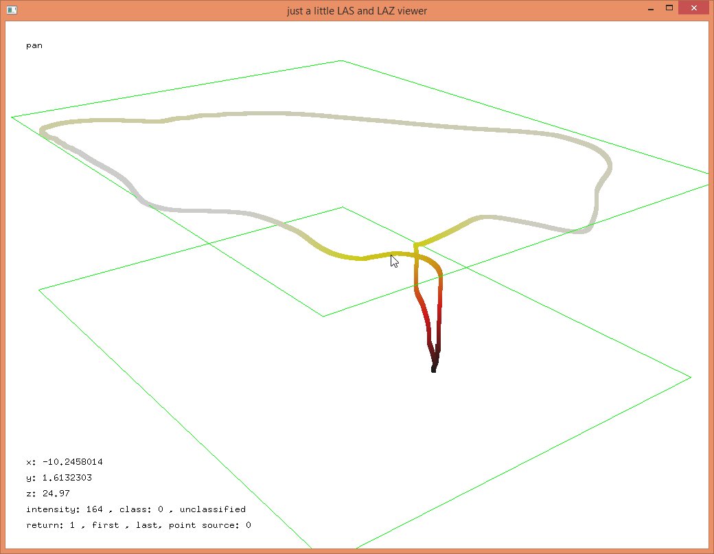
Using lasview and pressing <i> while hovering over those points of the trajectory that appear to be the survey start and end we determine visually that the timestamps between 164 to 264 correspond to the actual survey flight over the area of interest with the take-off and touch-down maneuvers excluded. We use las2las to cut out the relevant part and re-run lasgrid:

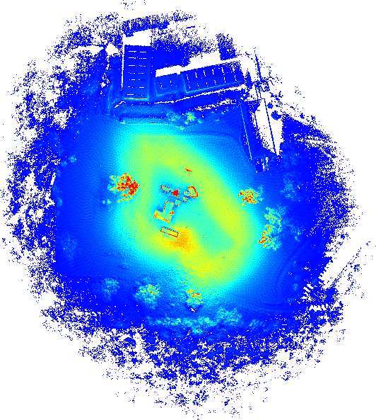
las2las -i CSIRO_Tower\results_fixed.laz ^
        -keep_gps_time 164 264 ^
        -o CSIRO_Tower\results_survey.laz

lasgrid -i CSIRO_Tower\results_survey.laz ^
        -last_only ^
        -step 0.5 -use_bb -density ^
        -false -set_min_max 0 1500 ^
        -o CSIRO_Tower\quality\density_0_1500_survey.png

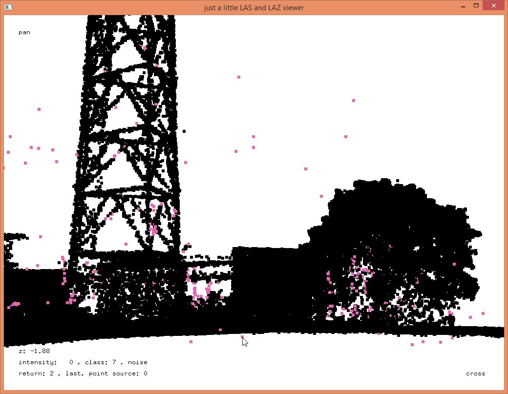
The other set of point we are less interested in are those occasional hits far from the scanner that sample the area too sparsely to be useful for anything. We use lastrack to reclassify points as noise (7) that exceed a x/y distance of 50 meters from the trajectory and then use lasgrid to create another density image without the points classified as noise..

lastrack -i CSIRO_Tower\results_survey.laz ^
         -track CSIRO_Tower\results_traj.laz ^
         -classify_xy_range_between 50 1000 7 ^
         -o CSIRO_Tower\results_xy50.laz

lasgrid -i CSIRO_Tower\results_xy50.laz ^
        -last_only -keep_class 0 ^
        -step 0.5 -use_bb -density ^
        -false -set_min_max 0 1500 ^
        -o CSIRO_Tower\quality\density_0_1500_xy50.png

We process the remaining points using a typical tile-based processing pipeline. First we run lastile to create tiling of 200 meter by 200 meter tiles with 20 buffers while dropping the noise points::

lastile -i CSIRO_Tower\results_xy50.laz ^
        -drop_class 7 ^
        -tile_size 200 -buffer 20 -flag_as_withheld ^
        -odir CSIRO_Tower\tiles_raw -o eta.laz

Because of the high sampling we expect there to be quite a few duplicate point where all three coordinate x, y, and z are identical. We remove them with a call to lasduplicate:

lasduplicate -i CSIRO_Tower\tiles_raw\*.laz ^
             -unique_xyz ^
             -odir CSIRO_Tower\tiles_unique -olaz ^
             -cores 4

This removes between 12 to 25 thousand point from each tile. Then we use lasnoise to classify isolated points as noise:

lasnoise -i CSIRO_Tower\tiles_unique\*.laz ^
         -step_xy 0.5 -step_z 0.1 -isolated 5 ^
         -odir CSIRO_Tower\tiles_denoised_temp -olaz ^
         -cores 4

This classifies between 13 to 23 thousand point from each tile into the noise classification code 7. We use rather aggressive settings to make sure we get most of the noise points that are below the terrain. Getting a correct ground classification in the next few steps is the main concern now even if this means that many points above the terrain on wires, towers, or vegetation will also get miss-classified as noise (at least temporarily). Next we use lasthin to classify a subset of points with classification code 8 on which we will then run the ground classification. We classify each point that is closest to the 5th percentile in elevation per 25 cm by 25 cm grid cell given there are at least 20 non-noise points in a cell. We then repeat this while increasing the cell size to 50 cm by 50 cm and 100 cm by 100 cm.

lasthin -i CSIRO_Tower\tiles_denoised_temp\*.laz ^
        -ignore_class 7 ^
        -step 0.25 -percentile 5 20 -classify_as 8 ^
        -odir CSIRO_Tower\tiles_thinned_025 -olaz ^
        -cores 4

lasthin -i CSIRO_Tower\tiles_thinned_025\*.laz ^
        -ignore_class 7 ^
        -step 0.50 -percentile 5 20 -classify_as 8 ^
        -odir CSIRO_Tower\tiles_thinned_050 -olaz ^
        -cores 4

lasthin -i CSIRO_Tower\tiles_thinned_025\*.laz ^
        -ignore_class 7 ^
        -step 1.00 -percentile 5 20 -classify_as 8 ^
        -odir CSIRO_Tower\tiles_thinned_100 -olaz ^
        -cores 4

 

Then we ground classify the points that were classified into the temporary classification code 8 in the previous step using lasground.

lasground -i CSIRO_Tower\tiles_thinned_100\*.laz ^
          -ignore_class 7 0 ^
          -town -ultra_fine ^
          -odir CSIRO_Tower\tiles_ground -olaz ^
          -cores 4

The resulting ground points are a lower envelope of the „fluffy“ sampled surfaces produced by the Velodyne Puck scanner. We use lasheight to thicken the ground by moving all points between 1 cm below and 6 cm above the TIN of these „low ground“ points to a temporary classification code 6 representing a „thick ground“. We also undo the overly aggressive noise classifications above the ground by setting all higher points back to classification code 1 (unclassified).

lasheight -i CSIRO_Tower\tiles_ground\*.laz ^
          -classify_between -0.01 0.06 6 ^
          -classify_above 0.06 1 ^
          -odir CSIRO_Tower\tiles_ground_thick -olaz ^
          -cores 4

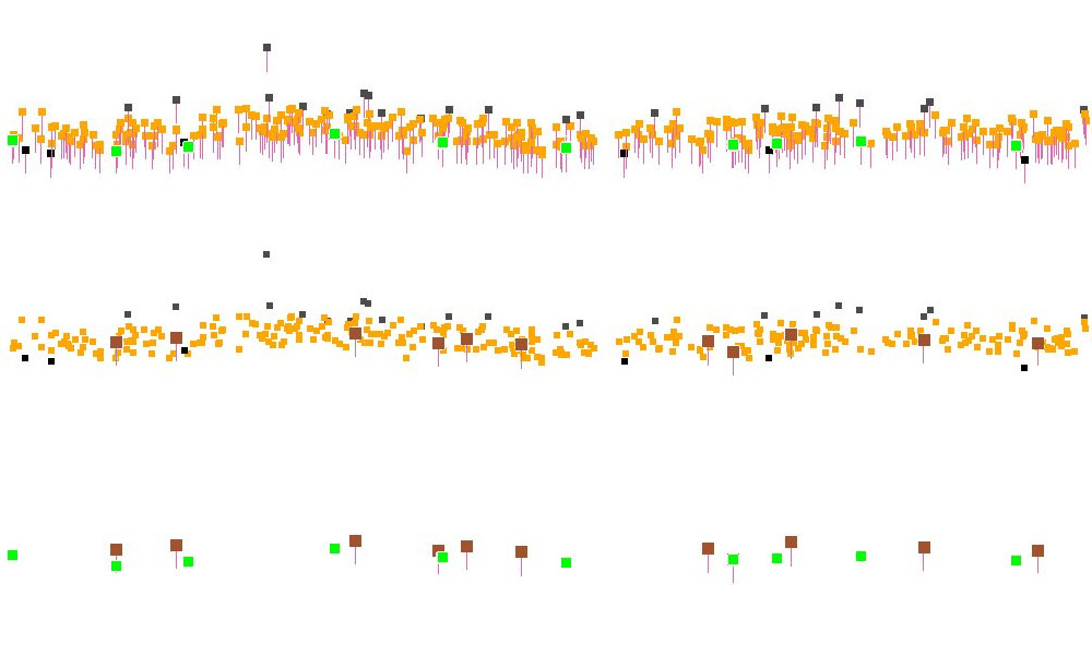
From the „thick ground“ we then compute a „median ground“ using lasthin in a similar fashion as we used it before. A profile view for a 25 centimeter wide strip of open terrain illustrates the workflow of going from „low ground“ via „thick ground“ to „median ground“ and shows the slight difference in elevation between the two.

lasthin -i CSIRO_Tower\tiles_ground_thick\*.laz ^
        -ignore_class 0 1 7 ^
        -step 0.25 -percentile 50 10 -classify_as 2 ^
        -odir CSIRO_Tower\tiles_ground_median_025 -olaz ^
        -cores 4

lasthin -i CSIRO_Tower\tiles_ground_median_025\*.laz ^
        -ignore_class 0 1 7 ^
        -step 0.50 -percentile 50 10 -classify_as 2 ^
        -odir CSIRO_Tower\tiles_ground_median_050 -olaz ^
        -cores 4

lasthin -i CSIRO_Tower\tiles_ground_median_050\*.laz ^
        -ignore_class 0 1 7 ^
        -step 1.00 -percentile 50 10 -classify_as 2 ^
        -odir CSIRO_Tower\tiles_ground_median_100 -olaz ^
        -cores 4

Then we use lasnoise once more with more conservative settings to remove the noise points that are sprinkled around the scene.

lasnoise -i CSIRO_Tower\tiles_ground_median_100\*.laz ^
         -step_xy 1.0 -step_z 1.0 -isolated 5 ^
         -odir CSIRO_Tower\tiles_denoised -olaz ^
         -cores 4

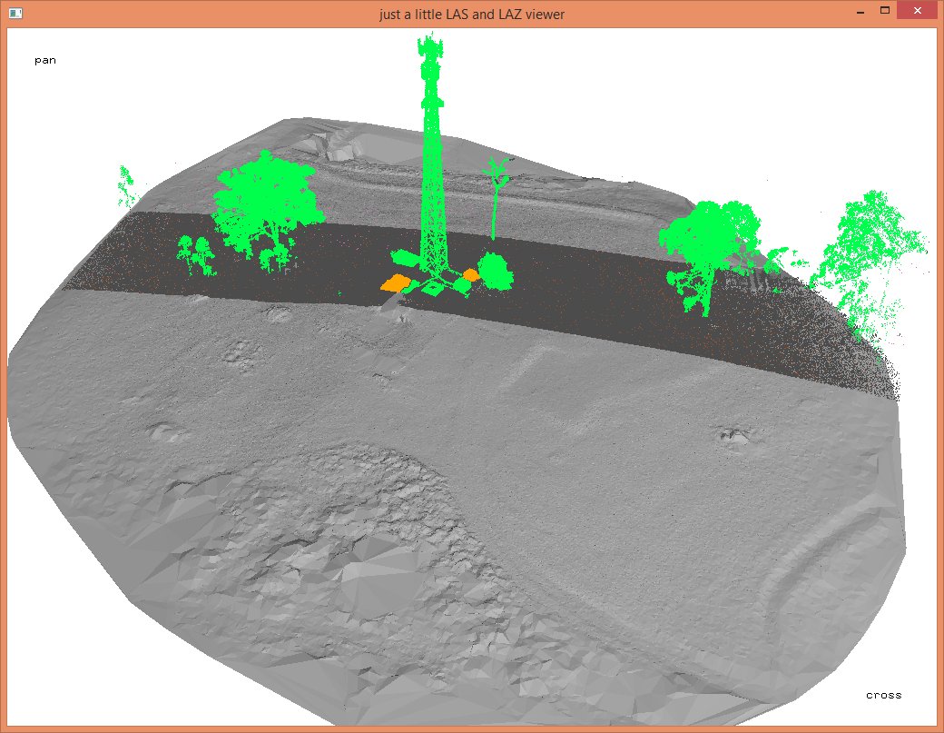
While we classify the scene into building roofs, vegetation, and everything else with lasclassify we also move all (unused) classifications to classification code 1 (unclassified). You may play with the parameters of lasclassify (see README) to achieve better a building classification. However, those buildings the laser can peek into (either via a window or because they are gazebo-like structures) will not be classified correctly. unless you remove the points that are under the roof somehow.

lasclassify -i CSIRO_Tower\tiles_denoised\*.laz ^
            -ignore_class 7 ^
            -change_classification_from_to 0 1 ^
            -change_classification_from_to 6 1 ^
            -step 1 ^
            -odir CSIRO_Tower\tiles_classified -olaz ^
            -cores 4

A glimpse at the final classification result is below. A hillshaded DTM and a strip of classified points. Of course the tower was miss-classified as vegetation given that it looks just like a tree to the logic used in lasclassify.

Finally we remove the tile buffers (that were really important for tile-based processing) with lastile:

lastile -i CSIRO_Tower\tiles_classified\*.laz ^
        -remove_buffer ^
        -odir CSIRO_Tower\tiles_final -olaz ^
        -cores 4

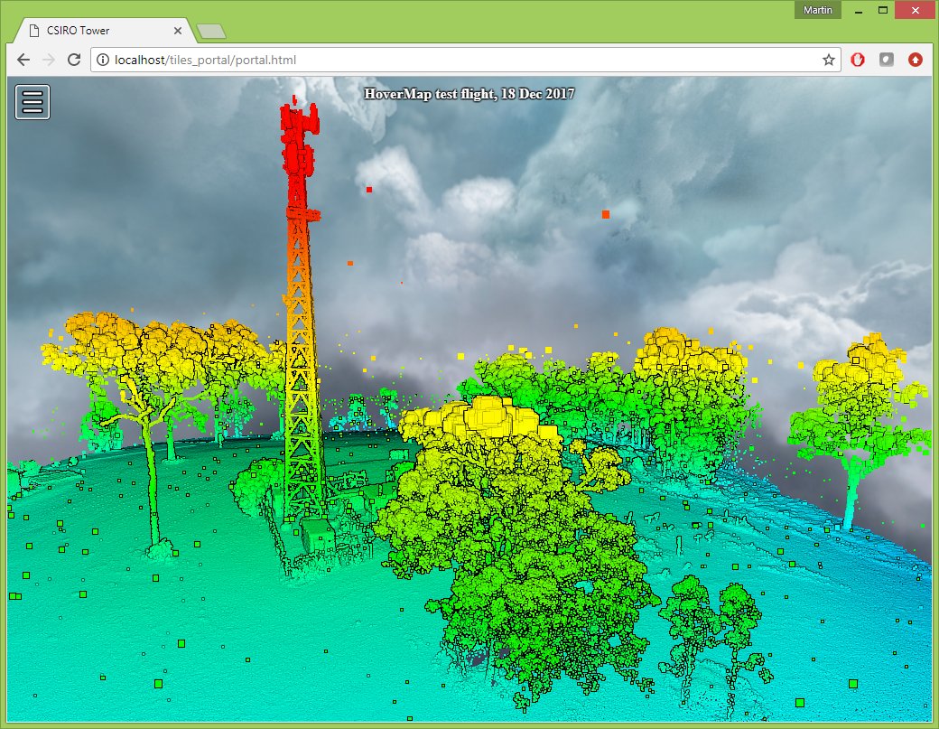
And publish the LiDAR point cloud as version 1.6 of Potree using laspublish:

laspublish -i CSIRO_Tower\tiles_final\*.laz ^
           -i CSIRO_Tower\results_traj.laz ^
           -only_3D -elevation -overwrite -potree16 ^
           -title "CSIRO Tower" ^
           -description "HoverMap test flight, 18 Dec 2017" ^
           -odir CSIRO_Tower\tiles_portal -o portal.html -olaz

Note that we also added the trajectory of the drone because it looks nice and gives a nice illustration of how the UAV was scanning the scene.

We would like to thank the entire team around Dr. Stefan Hrabar for taking time out of their busy schedules just a few days before Christmas.