Second German State Goes Open LiDAR

The floodgates of open geospatial data have opened in Germany. Days after reporting about the first state-wide release of open LiDAR, we are happy to follow up with a second wonderful open data story. The state of Thuringia (Thüringen) – also called the „green heart of Germany“ – has also implemented an open geospatial data policy. This had already been announced in March 2016 but must have gone online just now. A reader of our last blog article pointed this out in the comments. And it’s not just LiDAR. You can download:

• raster DTM (DGM) and DOM (DSM) and LiDAR points
• aerial images and orthophotos
• topographical maps (as GeoTIFFs or in layers)
• various land cover models
• shapefiles of all cadastral districts
• 3D buildings (LOD1 / LOD2) as CityGML
• building coordinates
• building footprints

It all comes with the same permissible license as OpenNRW’s data. This is open data madness! Everything you could possibly hope for presented via a very functional download portal. Kudos to TLVermGeo („Thüringisches Landesamt für Vermessung und Geoinformation“) for creating an open treasure cove of free-for-all geospatial data.

Let us have a look at the LiDAR. We use the interactive portal to zoom to an area of interest. With the recent rise of demagogues it cannot hurt to look at a stark reminder of where such demagoguery can lead. In his 1941 play „The Resistible Rise of Arturo Ui“ – a satirical allegory on the rise of Adolf Hitler – Bertolt Brecht writes „… don’t rejoice too soon at your escape. The womb he crawled from is still going strong.”

We are downloading LiDAR data around the Buchenwald concentration camp. According to Wikipedia, it was established in July 1937 and was one of the largest on German soil. Today the remains of Buchenwald serve as a memorial and as a permanent exhibition and museum.

We download the 15 tiles surrounding the blue one: two on its left, two on its right and one corresponding row of five tiles above and below. Each of the 15 zipped archives contains a *.laz file and *.meta file. The *.laz file contains the LiDAR points and *.meta file contains the textual information below where „Lage“ and „Höhe“ refer to „horizontal“ and „vertical“:

Datei: las_655_5653_1_th_2010-2013.laz
Erfassungsdatum: 2011-03
Erfassungsmethode: Airborne Laserscanning
Lasergebiet: Laser_04_2010
EPSG-Code Lage: 25832
EPSG-Code Höhe: 5783
Quasigeoid: GCG2005
Genauigkeit Lage: 0.12m
Genauigkeit Höhe: 0.04m
Urheber: (c) GDI-Th, Freistaat Thueringen, TLVermGeo

Next we will run a few quality checks on the 15 tiles by processing them with lasinfo, lasoverlap, lasgrid, and las2dem. We output all results into a folder named ‚quality‘.

With lasinfo we create one text file per tile that summarizes its contents. The ‚-cd‘ option computes the all return and last return density. The ‚-histo point_source 1‘ option produces a histogram of point source IDs that are supposed to store which flight line each return came from. The ‚-odir‘ and ‚-odix‘ options specify the directory for the output and an appendix to the output file name. The ‚-cores 4‘ option starts 4 processes in parallel, each working on a different tile.

lasinfo  -i las_*2010-2013.laz ^
         -cd ^
         -histo point_source 1 ^
         -odir quality -odix _info -otxt ^
         -cores 4

If you scrutinize the resulting text files you will find that the average last return density ranges from 6.29 to 8.13 and that the point source IDs 1 and 9999 seem to encode some special points. Likely those are synthetic points added to improve the derived rasters similar to the „ab“, „ag“, and „aw“ files in the OpenNRW LiDAR. Odd is the lack of intermediate returns despite return numbers ranging all the way up to 7. Looks like only the first returns and the last returns are made available (like for the OpenNRW LiDAR). That will make those a bit sad who were planning to use this LiDAR for forest or vegetation mapping. The header of the *.laz files does not store geo-referencing information, so we will have to enter that manually. And the classification codes do not follow the standard ASPRS assignment. In red is our (currently) best guess what these classification codes mean:

[...]
histogram of classification of points:
 887223 ground (2) ground
 305319 wire guard (13) building
 172 tower (15) bridges
 41 wire connector (16) synthetic ground under bridges
 12286 bridge deck (17) synthetic ground under building
 166 Reserved for ... (18) synthetic ground building edge
 5642801 Reserved for ... (20) non-ground
[...]

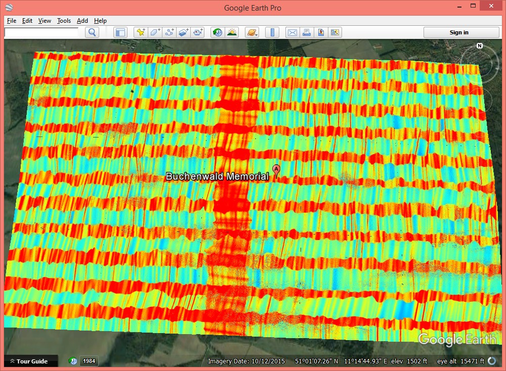
With lasoverlap we can visualize how much overlap the flight lines have and the (potential miss-)alignment between them. We drop the synthetic points with point source IDs 1 and 9999 and add geo-referencing information with ‚-epsg 25832‘ so that the resulting images can be displayed as Google Earth overlays. The options ‚-min_diff 0.1‘ and ‚-max_diff 0.4‘ map elevation differences of up +/- 10 cm to white. Above +/- 10 cm the color becomes increasingly red/blue with full saturation at +/- 40 cm or higher. This difference can only be computed for pixels with two or more overlapping flight lines.

lasoverlap  -i las_*2010-2013.laz ^
            -drop_point_source 1 ^
            -drop_point_source 9999 ^
            -min_diff 0.1 -max_diff 0.4 ^
            -odir quality -opng ^
            -epsg 25832 ^
            -cores 4

With lasgrid we check the density distribution of the laser pulses by computing the point density of the last returns for each 2 by 2 meter pixel and then mapping the computed density value to a false color that is blue for a density of 0 and red for a density of 10 or higher.

lasgrid  -i las_*2010-2013.laz ^
         -drop_point_source 1 ^
         -drop_point_source 9999 ^
         -keep_last ^
         -step 2 -point_density ^
         -false -set_min_max 0 10 ^
         -odir quality -odix _d_0_10 -opng ^
         -epsg 25832 ^
         -cores 4

With las2dem we can check the quality of the already existing ground classification in the LiDAR by producing a hillshaded image of a DTM for visual inspection. Based on our initial guess on the classification codes (see above) we keep those synthetic points that improve the DTM (classification codes 16, 17, and 18) in addition to the ground points (classification code 2).

las2dem  -i las_*2010-2013.laz ^
         -keep_class 2 16 17 18 ^
         -step 1 ^
         -hillshade ^
         -odir quality -odix _shaded_dtm -opng ^
         -epsg 25832 ^
         -cores 4

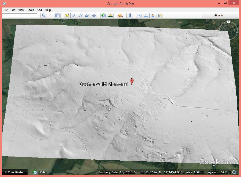
Wow. We see a number of ground disturbances in the resulting hillshaded DTM. Some of them are expected because if you read up on the history of the Buchenwald concentration camp you will learn that in 1950 large parts of the camp were demolished. However, the laser finds the remnants of those barracks and buildings as clearly visible ground disturbances under the canopy of the dense forest that has grown there since. And then there are also these bumps that look like bomb craters. Are those from the American bombing raid on August 24, 1944?

We are still not entirely sure what those „bumps“ arem but our initially assumption that all of those would have to be bomb craters from that fatal American bombing raid on August 24, 1944 seems to be wrong. Below is a close-up with lasview of the triangulated and shaded ground points from the lower right corner of tile ‚las_656_5654_1_th_2010-2013.laz‘.

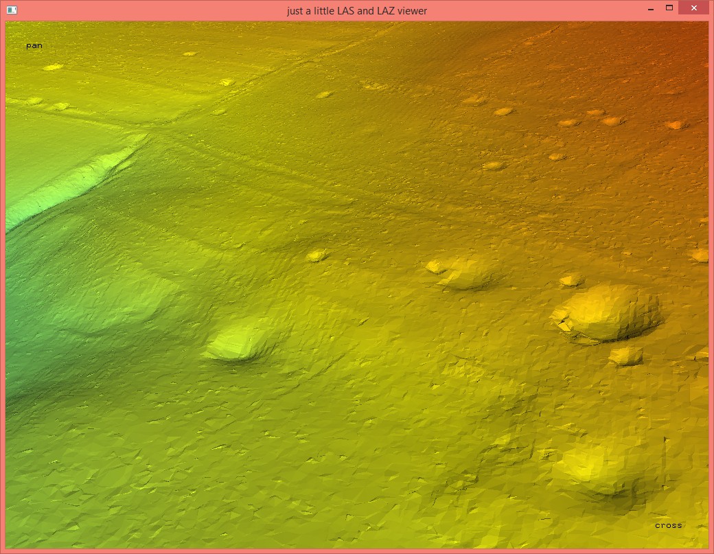
We are not sure if all the bumps we can see here are there for the same reason. But we found an old map and managed to overlay it on Google Earth. It suggest that at least the bigger bumps are not bomb craters. On the map they are labelled as „Erdfälle“ which is German for „sink hole“.

We got a reminder on the danger of demagogues as well as a glimpse into conflict archaeology and geomorphology with this open LiDAR download and processing exercise. If you want to explore this area any further you can either download the LiDAR and download LAStools and process the data yourself or simply get our KML files here.

Acknowledgement: The LiDAR data of TLVermGeo comes with a very permissible license. It is called “Datenlizenz Deutschland – Namensnennung – Version 2.0” or “dl-de/by-2-0” and allows data and derivative sharing as well as commercial use. It only requires us to name the source. We need to cite the “geoportal-th.de (2017)” with the year of the download in brackets and should specify the Universal Resource Identification (URI). We have not found this yet and use this URL as a placeholder until we know the correct one. Done. So easy. Thank you, geoportal Thüringen … (-: