We show how simple reordering and clever remapping of single photon LiDAR data can reduce file size by a whopping 50%. We also show that there is at least one Leica’s SPL100 sensor out there that should be called SPL99 because one of its 100 beamlets (the one with beamlet ID 53) does not seem to produce any data … (-:
Following up on a recent discussion in the LAStools user forum we take a closer look at some of the single photon LiDAR collected with Leica’s SPL100 sensor made available as open data by the USGS in form of LASzip-compressed tiles in LAS 1.4 format of point type 6. This investigation was sparked by the curiosity of what value was stored to the „scanner channel“ field that was added to the new point types 6 to 10 in the LAS 1.4 specification.
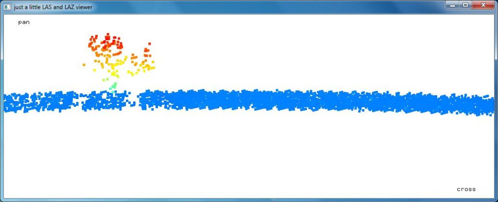
lasview -i USGS_LPC_SD_MORiver_Woolpert_B1_2016_14TNP120310_LAS_2018.laz ^
        -copy_scanner_channel_into_point_source ^
        -color_by_flightline
Visualizing this 2 bit number whose value can range from 0 to 3 for the first tile we downloaded resulted in this non-conclusive „magic eye“ visualization. What do you see? A sailboat?
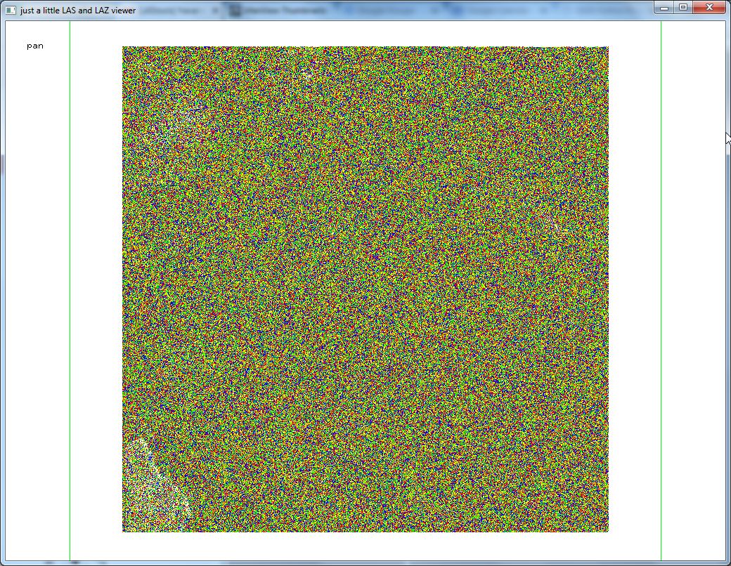
Jason Stoker from the USGS suggested that this is the truncated „beamlet“ ID. Leica’s SPL100 sensor uses 100 beamlets rather than one or two laser beams to collect data. Storing the beamlet IDs between 1 and 100 to this 2 bit field that can only hold numbers between 0 and 3 is kind of pointless and should be avoided. LASzip switches prediction contexts based on this field resulting in slower compression speed and lower compression rates. The beamlet ID is also stored in the 8 bit „user data“ field, so that we can simply zero the „scanner channel“ field. To investigate this further we downloaded these nine tiles from this FTP site of the USGS:
- USGS_LPC_SD_MORiver_Woolpert_B1_2016_14TNP120300_LAS_2018.laz
- USGS_LPC_SD_MORiver_Woolpert_B1_2016_14TNP120310_LAS_2018.laz
- USGS_LPC_SD_MORiver_Woolpert_B1_2016_14TNP120320_LAS_2018.laz
- USGS_LPC_SD_MORiver_Woolpert_B1_2016_14TNP130300_LAS_2018.laz
- USGS_LPC_SD_MORiver_Woolpert_B1_2016_14TNP130310_LAS_2018.laz
- USGS_LPC_SD_MORiver_Woolpert_B1_2016_14TNP130320_LAS_2018.laz
- USGS_LPC_SD_MORiver_Woolpert_B1_2016_14TNP140300_LAS_2018.laz
- USGS_LPC_SD_MORiver_Woolpert_B1_2016_14TNP140310_LAS_2018.laz
- USGS_LPC_SD_MORiver_Woolpert_B1_2016_14TNP140320_LAS_2018.laz
Whenever we download LAZ files we first run laszip with the ‚-check‘ option which performs a sanity check to make sure that the files are not truncated or otherwise corrupted. In our case we get nine solid reports of SUCCESS.
laszip -i USGS_LPC_SD_MORiver_Woolpert_B1_*_2018.laz -check
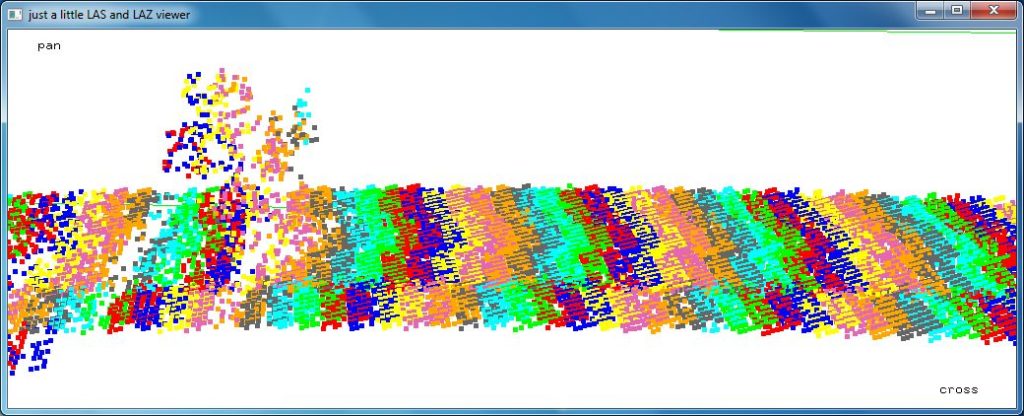
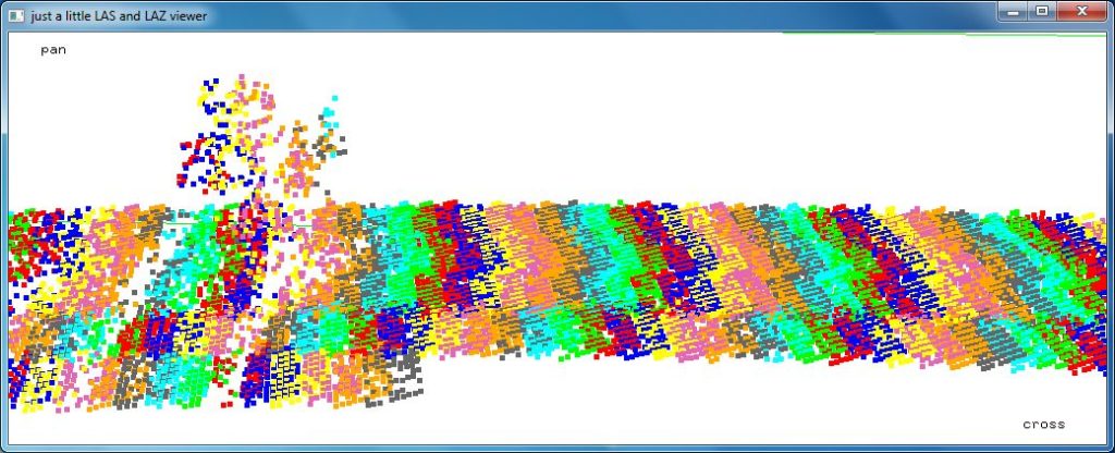
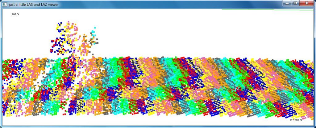
A visual inspection with lasview tells us that there are a number of flightlines in the data.
lasview -i USGS_LPC_SD_MORiver_Woolpert_B1_*_2018.laz ^
        -points 15000000 ^
        -color_by_flightline


We use las2las to extract flightline 2003 and lasinfo to produce a histogram of GPS times which we use in turn to decide on which quarter second of GPS time worth of data we want to extract again with las2las.
las2las -i USGS_LPC_SD_MORiver_Woolpert_B1_2016_*_LAS_2018.laz ^
        -merged ^
        -keep_point_source 2003 ^
        -o USGS_LPC_SD_MORiver_Woolpert_B1_ps_2002.laz

lasinfo -i USGS_LPC_SD_MORiver_Woolpert_B1_ps_2002.laz ^
        -cd ^
        -histo gps_time 1 ^
        -odix _info -otxt

las2las -i USGS_LPC_SD_MORiver_Woolpert_B1_ps_2002.laz ^
        -keep_gps_time 176475495 176475495.25 ^
        -o USGS_LPC_SD_MORiver_Woolpert_B1_gps176475495_quarter.laz
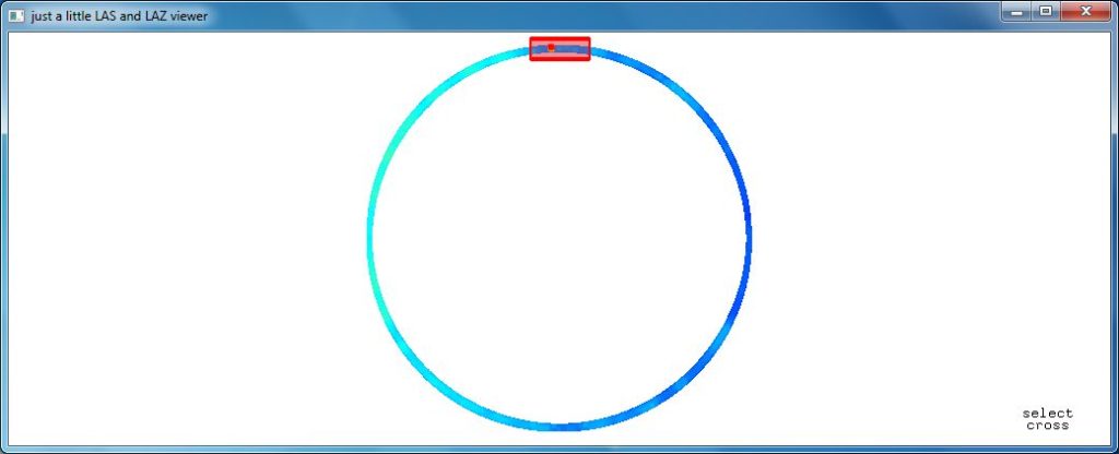
It always helps to give your LAZ files meaningful names in case you find them again two years later or so. We can nicely see the circular scanning pattern Leica’s SPL100 sensor. With lasview we measure that this single flightline has an extent of about 2000 meters on the ground. The lasinfo report shows a pulse density of around 19 last returns per square meter. We then sort the points by GPS time using lassort. This groups together all the returns that are the result of one „shot“ of the laser with 100 beamlets as we can nicely see in the las2txt output below. Each group of returns has slightly below 100 points and there is one group every 0.00002 seconds. This means the SPL100 is firing once every 20 microseconds.
lassort -i USGS_LPC_SD_MORiver_Woolpert_B1_gps176475495_quarter.laz ^
        -gps_time ^
        -odix _sorted -olaz

las2txt -i USGS_LPC_SD_MORiver_Woolpert_B1_gps176475495_quarter_sorted.laz ^
        -parse tuxyz ^
        -stdout | more
176475495.000008 4 514408.78 4830989.78 487.79
176475495.000008 9 514410.38 4830987.49 487.70
176475495.000008 47 514411.49 4830987.71 487.70
        [ ... 86 lines deleted ... ]
176475495.000008 39 514408.53 4830991.81 487.80
176475495.000008 50 514407.97 4830991.69 487.80
176475495.000008 16 514409.24 4830991.46 487.85
176475495.000028 55 514413.51 4830985.79 487.61
176475495.000028 97 514411.10 4830990.03 487.74
176475495.000028 72 514411.30 4830989.53 487.74
        [ ... 82 lines deleted ... ]
176475495.000028 45 514410.30 4830986.19 487.70
176475495.000028 3 514409.15 4830987.52 487.73
176475495.000028 96 514411.81 4830985.46 487.67
176475495.000048 66 514411.35 4830985.15 487.67
176475495.000048 83 514411.59 4830984.65 487.61
176475495.000048 64 514413.09 4830983.93 487.61
        [ ... 78 lines deleted ... ]
176475495.000048 4 514407.30 4830984.82 487.70
176475495.000048 34 514408.65 4830983.01 487.70
176475495.000048 21 514408.11 4830982.90 487.70
176475495.000068 13 514408.25 4830981.13 487.66
176475495.000068 92 514410.53 4830984.23 487.68
176475495.000068 44 514407.17 4830980.88 487.67
        [ ... 80 lines deleted ... ]
176475495.000068 76 514408.67 4830984.37 487.71
176475495.000068 47 514409.23 4830980.27 487.67
176475495.000068 87 514412.11 4830981.93 487.61
176475495.000088 97 514408.80 4830982.62 487.70
176475495.000088 33 514407.24 4830980.68 487.64
176475495.000088 30 514407.36 4830981.77 487.68
[ ... ]
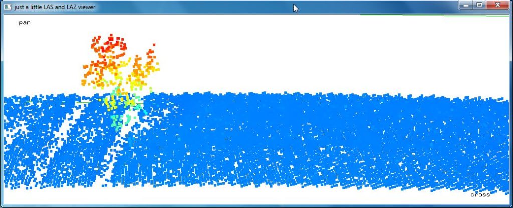
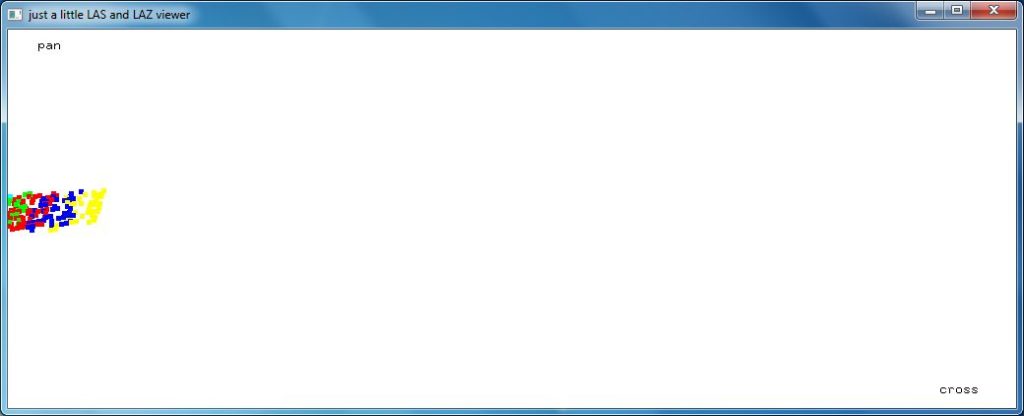
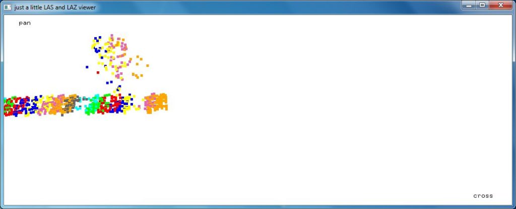
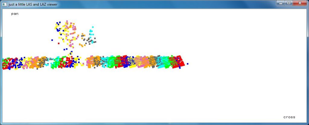
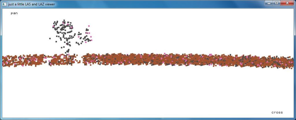
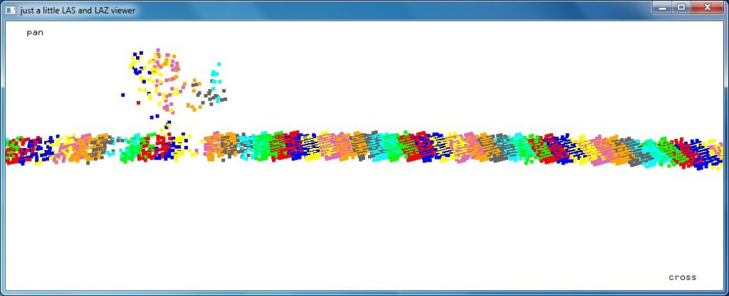
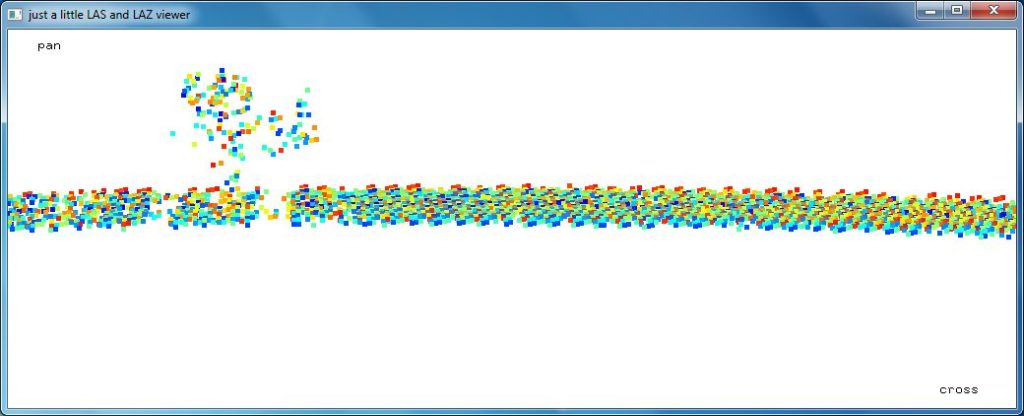
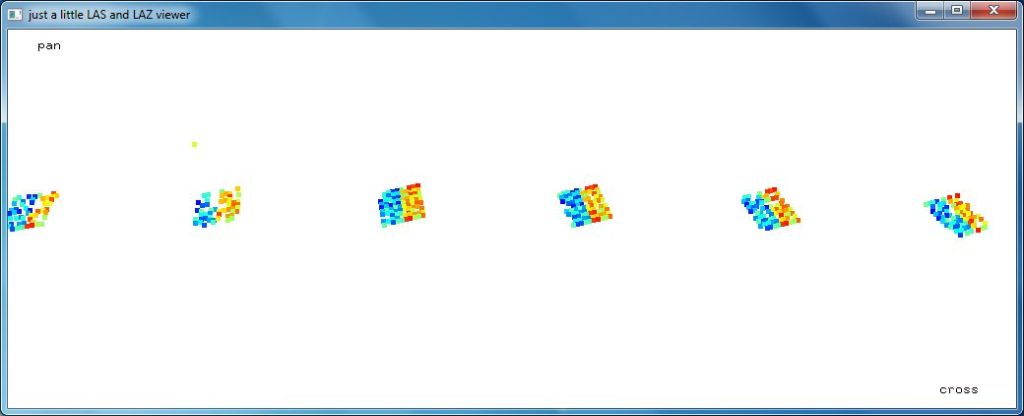
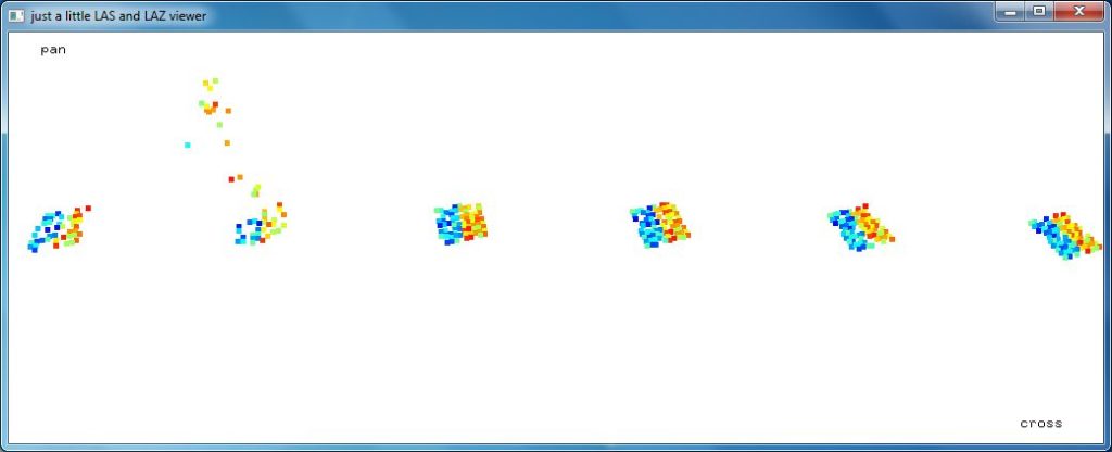
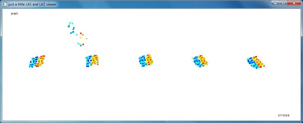
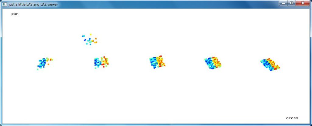
Now we can „play back“ the returns in acquisition order. We map returns from one group to the same color in lasview with the new ‚-bin_gps_time_into_point_source 0.00002‘ option (that will be available in the next LAStools release). For a slower playback we add ‚-steps 5000‘. Press the ‚c‘ key to switch through the coloring options. Press the ’s‘ key repeatedly to incrementally show the points. To take a step back press <SHIFT>+’s‘.
lasview -i USGS_LPC_SD_MORiver_Woolpert_B1_gps176475495_quarter_sorted.laz ^
        -bin_gps_time_into_point_source 0.00002 ^
        -scale_user_data 2.5 ^
        -steps 5000 ^
        -win 1024 384

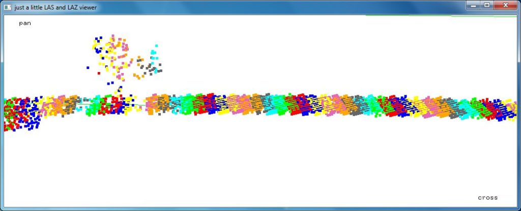
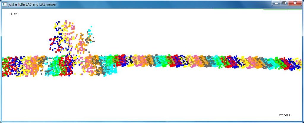


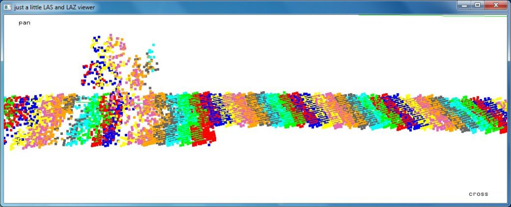

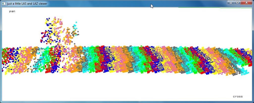
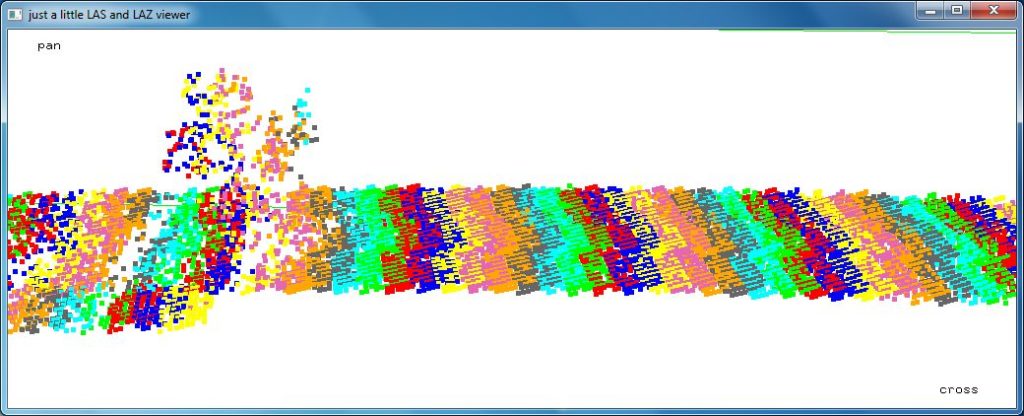


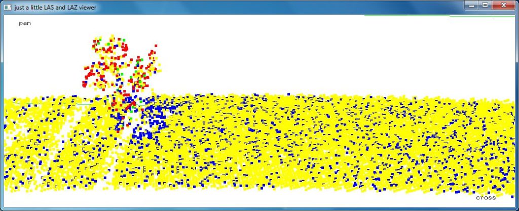


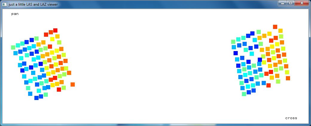
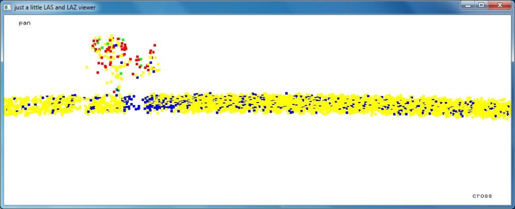
The last image colors the points by the values in the user data field (multiplied by 2.5), which essentially maps the beamlet IDs between 1 and 100 to a rainbow color ramp from blue to red. This tells us how the numbering of the beamlets from 1 to 100 corresponds to their layout in space. The next sequence of images takes a closer look at that.


From a compression point of view it makes sense to (1) zero the meaningless scanner channel, (2) order the points by GPS time stamps to groups beamlet returns together, and (3) order the points with the same time stamp by the user data field. The compression gain is enormous with the 9 tiles going from over 3 GB to under 2 GB:
ORIGINAL:
337,156,981 USGS_LPC_SD_MORiver_Woolpert_B1_2016_14TNP120300_LAS_2018.laz
331,801,150 USGS_LPC_SD_MORiver_Woolpert_B1_2016_14TNP120310_LAS_2018.laz
358,928,274 USGS_LPC_SD_MORiver_Woolpert_B1_2016_14TNP120320_LAS_2018.laz
328,597,628 USGS_LPC_SD_MORiver_Woolpert_B1_2016_14TNP130300_LAS_2018.laz
355,997,013 USGS_LPC_SD_MORiver_Woolpert_B1_2016_14TNP130310_LAS_2018.laz
360,403,079 USGS_LPC_SD_MORiver_Woolpert_B1_2016_14TNP130320_LAS_2018.laz
355,399,781 USGS_LPC_SD_MORiver_Woolpert_B1_2016_14TNP140300_LAS_2018.laz
354,523,659 USGS_LPC_SD_MORiver_Woolpert_B1_2016_14TNP140310_LAS_2018.laz
357,248,968 USGS_LPC_SD_MORiver_Woolpert_B1_2016_14TNP140320_LAS_2018.laz
  3,140,056,533 Bytes

IMPROVED:
197,641,087 USGS_LPC_SD_MORiver_Woolpert_B1_2016_14TNP120300_LAS_2018_sorted.laz
194,750,096 USGS_LPC_SD_MORiver_Woolpert_B1_2016_14TNP120310_LAS_2018_sorted.laz
210,013,408 USGS_LPC_SD_MORiver_Woolpert_B1_2016_14TNP120320_LAS_2018_sorted.laz
190,687,275 USGS_LPC_SD_MORiver_Woolpert_B1_2016_14TNP130300_LAS_2018_sorted.laz
206,447,730 USGS_LPC_SD_MORiver_Woolpert_B1_2016_14TNP130310_LAS_2018_sorted.laz
209,580,551 USGS_LPC_SD_MORiver_Woolpert_B1_2016_14TNP130320_LAS_2018_sorted.laz
205,827,197 USGS_LPC_SD_MORiver_Woolpert_B1_2016_14TNP140300_LAS_2018_sorted.laz
203,808,113 USGS_LPC_SD_MORiver_Woolpert_B1_2016_14TNP140310_LAS_2018_sorted.laz
206,789,959 USGS_LPC_SD_MORiver_Woolpert_B1_2016_14TNP140320_LAS_2018_sorted.laz
  1,825,545,416 Bytes
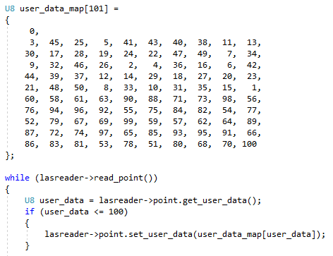
Enumerating the 100 beamlets with a geometrically more coherent order would improve compression even more. Can anyone convince Leica to do this? The simple mapping of beamlet IDs shown below that arranges the beamlets into a zigzag order another huge compression gain of 15 percent. Altogether reordering and remapping lower the compressed file size by a whopping 50 percent.
168,876,666 USGS_LPC_SD_MORiver_Woolpert_B1_2016_14TNP120300_LAS_2018_mapped_sorted.laz
165,241,508 USGS_LPC_SD_MORiver_Woolpert_B1_2016_14TNP120310_LAS_2018_mapped_sorted.laz
176,524,959 USGS_LPC_SD_MORiver_Woolpert_B1_2016_14TNP120320_LAS_2018_mapped_sorted.laz
163,679,216 USGS_LPC_SD_MORiver_Woolpert_B1_2016_14TNP130300_LAS_2018_mapped_sorted.laz
176,086,559 USGS_LPC_SD_MORiver_Woolpert_B1_2016_14TNP130310_LAS_2018_mapped_sorted.laz
178,909,108 USGS_LPC_SD_MORiver_Woolpert_B1_2016_14TNP130320_LAS_2018_mapped_sorted.laz
174,735,634 USGS_LPC_SD_MORiver_Woolpert_B1_2016_14TNP140300_LAS_2018_mapped_sorted.laz
171,679,105 USGS_LPC_SD_MORiver_Woolpert_B1_2016_14TNP140310_LAS_2018_mapped_sorted.laz
174,997,090 USGS_LPC_SD_MORiver_Woolpert_B1_2016_14TNP140320_LAS_2018_mapped_sorted.laz
  1,550,729,845 Bytes
Once this is done a final space-filling sort into a Hilbert-curve or a Morton-order with lassort or lasoptimize would improve spatial coherence for efficient spatial indexing with lasindex.
Oh yes … the SPL100 was not firing on all cylinders. The beamlet ID 53 that would have mapped to 61 in our table was not present in any of the 9 tiles with 355,047,478 points that we had downloaded as the lasinfo histogram below shows.
lasinfo -i USGS_LPC_SD_MORiver_Woolpert_B1_2016_*_2018.laz -merged -histo user_data 1
lasinfo (180911) report for 9 merged files
reporting all LAS header entries:
  file signature:             'LASF'
  file source ID:             0
  global_encoding:            17
  project ID GUID data 1-4:   194774FA-35FE-4591-D484-010AFA13F6D9
  version major.minor:        1.4
  system identifier:          'Woolpert LAS'
  generating software:        'GeoCue LAS Updater'
  file creation day/year:     332/2017
  header size:                375
  offset to point data:       1376
  number var. length records: 1
  point data format:          6
  point data record length:   30
  number of point records:    0
  number of points by return: 0 0 0 0 0
  scale factor x y z:         0.01 0.01 0.01
  offset x y z:               0 0 0
  min x y z:                  512000.00 4830000.00 286.43
  max x y z:                  514999.99 4832999.99 866.81
  start of waveform data packet record: 0
  start of first extended variable length record: 0
  number of extended_variable length records: 0
  extended number of point records: 355047478
  extended number of points by return: 298476060 52480771 3929583 157365 3699 0 0 0 0 0 0 0 0 0 0
variable length header record 1 of 1:
  reserved             0
  user ID              'LASF_Projection'
  record ID            2112
  length after header  943
  description          'OGC WKT Coordinate System'
    WKT OGC COORDINATE SYSTEM:
    COMPD_CS["NAD83(2011) / UTM zone 14N + NAVD88 height - Geoid12B (metre)",PROJCS["NAD83(2011) / UTM zone 14N",GEOGCS["NAD83(2011)",DATUM["NAD83_National_Spat
ial_Reference_System_2011",SPHEROID["GRS 1980",6378137,298.257222101,AUTHORITY["EPSG","7019"]],AUTHORITY["EPSG","1116"]],PRIMEM["Greenwich",0,AUTHORITY["EPSG","
8901"]],UNIT["degree",0.0174532925199433,AUTHORITY["EPSG","9122"]],AUTHORITY["EPSG","6318"]],PROJECTION["Transverse_Mercator"],PARAMETER["latitude_of_origin",0]
,PARAMETER["central_meridian",-99],PARAMETER["scale_factor",0.9996],PARAMETER["false_easting",500000],PARAMETER["false_northing",0],UNIT["metre",1,AUTHORITY["EP
SG","9001"]],AXIS["Easting",EAST],AXIS["Northing",NORTH],AUTHORITY["EPSG","6343"]],VERT_CS["NAVD88 height - Geoid12B (metre)",VERT_DATUM["North American Vertica
l Datum 1988",2005,AUTHORITY["EPSG","5103"]],UNIT["metre",1,AUTHORITY["EPSG","9001"]],AXIS["Gravity-related height",UP],AUTHORITY["EPSG","5703"]]]
the header is followed by 4 user-defined bytes
LASzip compression (version 3.1r0 c3 50000): POINT14 3
reporting minimum and maximum for all LAS point record entries ...
  X            51200000   51499999
  Y           483000000  483299999
  Z               28643      86681
  intensity        3139      12341
  return_number       1          5
  number_of_returns   1          5
  edge_of_flight_line 0          0
  scan_direction_flag 0          1
  classification      1         10
  scan_angle_rank  -127        127
  user_data           1        100
  point_source_ID  1061       2005
  gps_time 176475467.194000 176496233.636563
  extended_return_number          1      5
  extended_number_of_returns      1      5
  extended_classification         1     10
  extended_scan_angle        -21167  21167
  extended_scanner_channel        0      3
number of first returns:        298476060
number of intermediate returns: 6282
number of last returns:         355000765
number of single returns:       298435629
overview over extended number of returns of given pulse: 298435629 52515017 3935373 157750 3709 0 0 0 0 0 0 0 0 0 0
histogram of classification of points:
       138382030  unclassified (1)
       207116732  ground (2)
         9233160  noise (7)
          310324  water (9)
            5232  rail (10)
 +-> flagged as withheld:  9233160
 +-> flagged as extended overlap: 226520346
user data histogram with bin size 1.000000
  bin 1 has 3448849
  bin 2 has 3468566
  bin 3 has 3721848
  bin 4 has 3376990
  bin 5 has 3757996
  bin 6 has 3479546
  bin 7 has 3799930
  bin 8 has 3766887
  bin 9 has 3448383
  bin 10 has 3966036
  bin 11 has 3232086
  bin 12 has 3686789
  bin 13 has 3763869
  bin 14 has 3847765
  bin 15 has 3659059
  bin 16 has 3666918
  bin 17 has 3427468
  bin 18 has 3375320
  bin 19 has 3222116
  bin 20 has 3598643
  bin 21 has 3108323
  bin 22 has 3553625
  bin 23 has 3782185
  bin 24 has 3577792
  bin 25 has 3063871
  bin 26 has 3451800
  bin 27 has 3518763
  bin 28 has 3845852
  bin 29 has 3366980
  bin 30 has 3797986
  bin 31 has 3623477
  bin 32 has 3606798
  bin 33 has 3762737
  bin 34 has 3861023
  bin 35 has 3821228
  bin 36 has 3738173
  bin 37 has 3902190
  bin 38 has 3726752
  bin 39 has 3910989
  bin 40 has 3771132
  bin 41 has 3718437
  bin 42 has 3609113
  bin 43 has 3339941
  bin 44 has 3003191
  bin 45 has 3697140
  bin 46 has 2329171
  bin 47 has 3398836
  bin 48 has 3511882
  bin 49 has 3719592
  bin 50 has 2995275
  bin 51 has 3673925
  bin 52 has 3535992
  bin 54 has 3799430
  bin 55 has 3613345
  bin 56 has 3761436
  bin 57 has 3296831
  bin 58 has 3810146
  bin 59 has 3768464
  bin 60 has 3520871
  bin 61 has 3833149
  bin 62 has 3639778
  bin 63 has 3623008
  bin 64 has 3581480
  bin 65 has 3663180
  bin 66 has 3661434
  bin 67 has 3684374
  bin 68 has 3723125
  bin 69 has 3552397
  bin 70 has 3554207
  bin 71 has 3535494
  bin 72 has 3621334
  bin 73 has 3633928
  bin 74 has 3631845
  bin 75 has 3526502
  bin 76 has 3605631
  bin 77 has 3452006
  bin 78 has 3796382
  bin 79 has 3731841
  bin 80 has 3683314
  bin 81 has 3806024
  bin 82 has 3749709
  bin 83 has 3808218
  bin 84 has 3634032
  bin 85 has 3631015
  bin 86 has 3712206
  bin 87 has 3627775
  bin 88 has 3674966
  bin 89 has 3231151
  bin 90 has 3780037
  bin 91 has 3621958
  bin 92 has 3623264
  bin 93 has 3853536
  bin 94 has 3623380
  bin 95 has 3418309
  bin 96 has 3374827
  bin 97 has 3464734
  bin 98 has 3562560
  bin 99 has 3078686
  bin 100 has 3426924
Pingback: Removing Noise from Single Photon LiDAR to Generate a Smooth DTM | rapidlasso GmbH