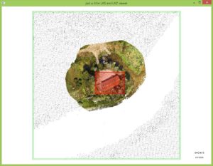
We collected drone imagery of the restored „Kance“ tavern during the lunch stop of the UAV Tartu summer school field trip (actually the organizer Marko Kohv did that, as I was busy introducing students to SUP boarding). With Agisoft PhotoScan we then processed the images into point clouds below the deck of the historical „Jõmmu“ barge on the way home (actually Marko did that, because I was busy enjoying the view of the wetlands in the afternoon sun). The resulting data set with 7,855,699 points is shown below and can be downloaded here.

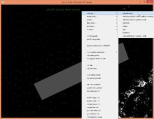
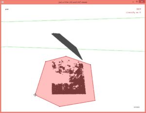
Generating points using photogrammetric techniques in scenes containing water bodies tends to be problematic as dense blotches of noise points above and below the water surface are common as you can see in the picture below. Especially the low points are troublesome as they adversely affect ground classification which results in poor Digital Elevation Models (DTMs).

In a previous article we have described a LAStools workflow that can remove excessive low noise. In this article here we use external information about the topography of the area to clean our photogrammetry points. How convenient that the Estonian Land Board has just released their entire LiDAR archives as open data.
Following these instructions here you can download the available open LiDAR for this area, which has the map sheet index 475681. Alternatively you can download the four currently available data sets here flown in spring 2010, in summer 2013, in spring 2014, and in summer 2017. In the following we will use the one flown in spring 2014.
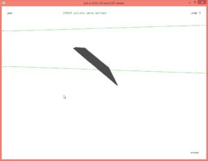
We can view both data sets simultaneously in lasview. By adding ‚-faf‘ to the command-line we can switch back and forth between the two data sets by pressing ‚0‘ and ‚1‘.
lasview -i Kantsi.laz ^
        -i 475681_2014_tava.laz ^
        -points 10000000 ^
        -faf
We find cut the 1 km by 1 km LiDAR tile down to a 250 m by 250 m tile that nicely surrounds our photogrammetric point set using the following las2las command-line:
las2las -i 475681_2014_tava.laz ^
        -inside_tile 681485 6475375 250 ^
        -o LiDAR_Kantsi.laz

lasview -i Kantsi.laz ^
        -i LiDAR_Kantsi.laz ^
        -points 10000000 ^
        -faf
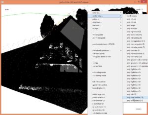
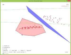
Scrutinizing the two data sets we quickly find that there is a miss-alignment between the dense imagery-derived and the comparatively sparse LiDAR point clouds. With lasview we investigate the difference between the two point clouds by hovering over a point from one point cloud and pressing <i> and then hovering over a somewhat corresponding point from the other point cloud and pressing <SHIFT>+<i>. We measure displacements of around 2 meters vertically and of around 3 to 3.5 meter in total.


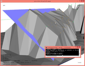
Before we can use the LiDAR points to remove the low noise from the photogrammetric points we must align them properly. For simple translation errors this can be done with a new feature that was recently added to lasview. Make sure to download the latest version (190404 or newer) of LAStools to follow the steps shown in the image sequence below.


las2las -i Kantsi.laz ^
        -translate_xyz 0.89 -1.90 2.51 ^
        -o Kantsi_shifted.laz

lasview -i Kantsi_shifted.laz ^
        -i LiDAR_Kantsi.laz ^
        -points 10000000 ^
        -faf
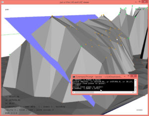
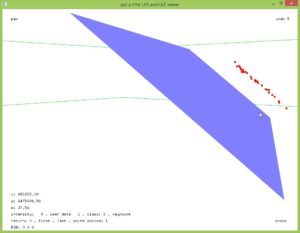
The result looks good in the sense that both sides of the photogrammetric roof are reasonably well aligned with the LiDAR. But there is still a shift along the roof so we repeat the same thing once more as shown in the next image sequence:
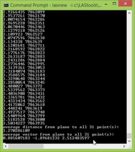
We use a suitable displacement vector and apply it to the photogrammetry points, shifting them again:
las2las -i Kantsi_shifted.laz ^
        -translate_xyz -1.98 -0.95 0.01 ^
        -o Kantsi_shifted_again.laz

lasview -i Kantsi_shifted_again.laz ^
        -i LiDAR_Kantsi.laz ^
        -points 10000000 ^
        -faf
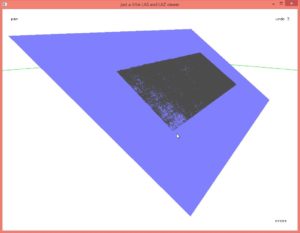
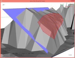
The result is still not perfect as there is also some rotational error and you may find another software such as Cloud Compare more suited to align the two point clouds, but for this exercise the alignment shall suffice. Below you see the match between the photogrammetry points and the LiDAR TIN before and after shifting the photogrammetry points with the two (interactively determined) displacement vectors.
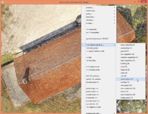
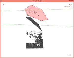
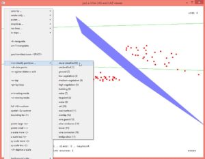
The final steps of this exercise use las2dem and the already ground-classified LiDAR compute a 1 meter DTM, which we then use as input to lasheight. We classify the photogrammetry points using their height above this set of ground points with 1 meter spacing: points that are 40 centimeter or more below the LiDAR DTM are classified as noise (7), points that are between 40 below to 1 meter above the LiDAR DTM are classified to a temporary class (here we choose 8) that has those points that could potentially be ground points. This will help, for example, with subsequent ground classification as large parts of the photogrammetry points – namely those on top of buildings and in higher vegetation – can be ignored from the start by a ground classification algorithm such as lasground.
las2dem -i LiDAR_Kantsi.laz ^
        -keep_class 2 ^
        -kill 1000 ^
        -o LiDAR_Kantsi_dtm_1m.bil
lasheight -i Kantsi_shifted_again.laz ^
          -ground_points LiDAR_Kantsi_dtm_1m.bil ^
          -classify_below -0.4 7 ^
          -classify_between -0.4 1.0 8 ^
          -o Kantsi_cleaned.laz
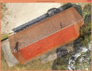
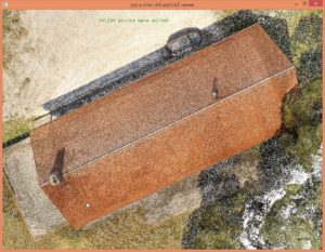
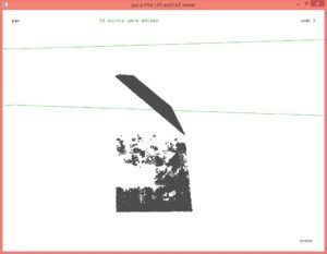
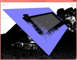
Below the results we have achieved after „roughly“ aligning the two point clouds with some new lasview tricks and then using the LiDAR elevations to classify the photogrammetry points into „low noise“, „potential ground“, and „all else“.
We thank the Estonian Land Board for providing open data with a permissive license. Special thanks also go to the organizers of the UAV Summer School in Tartu, Estonia and the European Regional Development Fund for funding this event. Especially fun was the fabulous excursion to the Emajõe-Suursoo Nature Reserve and through to Lake Peipus aboard, overboard and aboveboard the historical barge „Jõmmu“. If you look carefully you can also find the barge in the photogrammetry point cloud. The photogrammetry data used here was acquired during our lunch stop.
