New Step-by-Step Tutorial for Velodyne Drone LiDAR from Snoopy by LidarUSA

The folks from Harris Aerial gave us LiDAR data from a test-flight of one of their drones, the Carrier H4 Hybrid HE (with a 5kg maximum payload and a retail price of US$ 28,000), carrying a Snoopy A series LiDAR system from LidarUSA in the countryside near Huntsville, Alabama. The laser scanner used by the Snoopy A series is a Velodyne HDL 32E that has 32 different laser/detector pairs that fire in succession to scan up to 700,000 points per second within a range of 1 to 70 meters. You can download the raw LiDAR file from the 80 second test flight here. As always, the first thing we do is to visualize the file with lasview and to generate a textual report of its contents with lasinfo.

lasview -i Velodyne001.laz -set_min_max 680 750

It becomes obvious that the drone must have scanned parts of itself (probably the landing gear) during the flight and we exploit this fact in the later processing. The information which of the 32 lasers was collecting which point is stored into the ‚point source ID‘ field which is usually used for the flightline information. This results in a psychedelic look in lasview as those 32 different numbers get mapped to the 8 different colors that lasview uses for distinguishing flightlines.

The lasinfo report we generate computes the average point density with ‚-cd‘ and includes histograms for a number of point attributes, namely for ‚user data‘, ‚intensity‘, ‚point source ID‘, ‚GPS time‘, and ’scan angle rank‘.

lasinfo -i Velodyne001.laz ^
        -cd ^
        -histo user_data 1 ^
        -histo point_source 1 ^
        -histo intensity 16 ^
        -histo gps_time 1 ^
        -histo scan_angle_rank 5 ^
        -odir quality -odix _info -otxt

You can download the resulting report here and it will tell you that the information which of the 32 lasers was collecting which point was stored both into the ‚user data‘ field and into the ‚point source ID‘ field. The warnings you see below have to do with the fact that the double-precision bounding box stored in the LAS header was populated with numbers that have many more decimal digits than the coordinates in the file, which only have millimeter (or millifeet) resolution as all three scale factors are 0.001 (meaning three decimal digits).

WARNING: stored resolution of min_x not compatible with x_offset and x_scale_factor: 2171988.6475160527
WARNING: stored resolution of min_y not compatible with y_offset and y_scale_factor: 1622812.606925504
WARNING: stored resolution of min_z not compatible with z_offset and z_scale_factor: 666.63504345017589
WARNING: stored resolution of max_x not compatible with x_offset and x_scale_factor: 2172938.973065129
WARNING: stored resolution of max_y not compatible with y_offset and y_scale_factor: 1623607.5209975131
WARNING: stored resolution of max_z not compatible with z_offset and z_scale_factor: 1053.092674726669

Both the „return number“ and the „number of returns“ attribute of every points in the file is 2. This makes it appear as if the file would only contain the last returns of those laser shots that produced two returns. However, as the Velodyne HDL 32E only produces one return per shot we can safely conclude that those numbers should all be 1 instead of 2 and that this is just a small bug in the export software. We can easily fix this with las2las.

reporting minimum and maximum for all LAS point record entries ...
[...]
 return_number 2 2
 number_of_returns 2 2
[...]

The lasinfo report lacks information about the coordinate reference system as there is no VLR that stores projection information. Harris Aerial could not help us other than telling us that the scan was near Huntsville, Alamaba. Measuring certain distances in the scene like the height of the house or the tree suggests that both horizontal and vertical units are in feet, or rather in US survey feet. After some experimenting we find that using EPSG 26930 for NAD83 Alabama West but forcing the default horizontal units from meters to US survey feet gives a result that aligns well with high-resolution Google Earth imagery as you can see below:

lasgrid -i flightline1.laz ^
        -i flightline2.laz ^
        -merged ^
        -epsg 26930 -survey_feet ^
        -step 1 -highest ^
        -false -set_min_max 680 750 ^
        -o testing26930usft.png

We use the fact that the drone has scanned itself to extract an (approximate) trajectory by isolating those LiDAR returns that have hit the drone. Via a visual check with lasview (by hovering with the cursor over the lowest drone hits and pressing hotkey ‚i‘) we determine that the lowest drone hits are all above 719 feet. We use two calls to las2las to split the point cloud vertically. In the same call we also change the resolution from three to two decimal digits, fix the return number issue, and add the missing geo-referencing information:

las2las -i Velodyne001.laz ^
        -rescale 0.01 0.01 0.01 ^
        -epsg 26930 -survey_feet -elevation_survey_feet ^
        -set_return_number 1 ^
        -set_number_of_returns 1 ^
        -keep_z_above 719 ^
        -odix _above719 -olaz

las2las -i Velodyne001.laz ^
        -rescale 0.01 0.01 0.01 ^
        -epsg 26930 -survey_feet -elevation_survey_feet ^
        -set_return_number 1 ^
        -set_number_of_returns 1 ^
        -keep_z_below 719 ^
        -odix _below719 -olaz

We then use the manual editing capabilities of lasview to change the classifications of the LiDAR points that correspond to drone hits from 1 to 12, which is illustrated by the series of screen shots below.

lasview -i Velodyne001_above719.laz

The workflow illustrated above results in a tiny LAY file that is part of the LASlayers functionality of LAStools. It only encodes the few changes in classifications that we’ve made to the LAZ file without re-writing those parts that have not changed. Those interested may use laslayers to inspect the structure of the LAY file:

laslayers -i Velodyne001_above719.laz

We can apply the LAY file on-the-fly with the ‚-ilay‘ option, for example, when running lasview:

lasview -i Velodyne001_above719.laz -ilay

To separate the drone-hit trajectory from the remaining points we run lassplit with the ‚-ilay‘ option and request to split by classification with this command line:

lassplit -i Velodyne001_above719.laz -ilay ^
         -by_classification -digits 3 ^
         -olaz

This gives us two new files with the three-digit appendices ‚_001‘ and ‚_012‘. The latter one contains those points we marked as being part of the trajectory. We now want to use lasview to – visually – find a good moment in time where to split the trajectory into multiple flightlines. The lasinfo report tells us that the GPS time stamps are in the range from 418,519 to 418,602. In order to use the same trick as we did in our recent article on processing LiDAR data from the Hovermap Drone, where we mapped the GPS time to the intensity for querying it via lasview, we first need to subtract a large number from the GPS time stamps to bring them into a suitable range that fits the intensity field as done here.

lasview -i Velodyne001_above719_012.laz ^
        -translate_gps_time -418000 ^
        -bin_gps_time_into_intensity 1
        -steps 5000

The ‚-steps 5000‘ argument makes for a slower playback (press ‚p‘ to repeat) to better follow the trajectory.

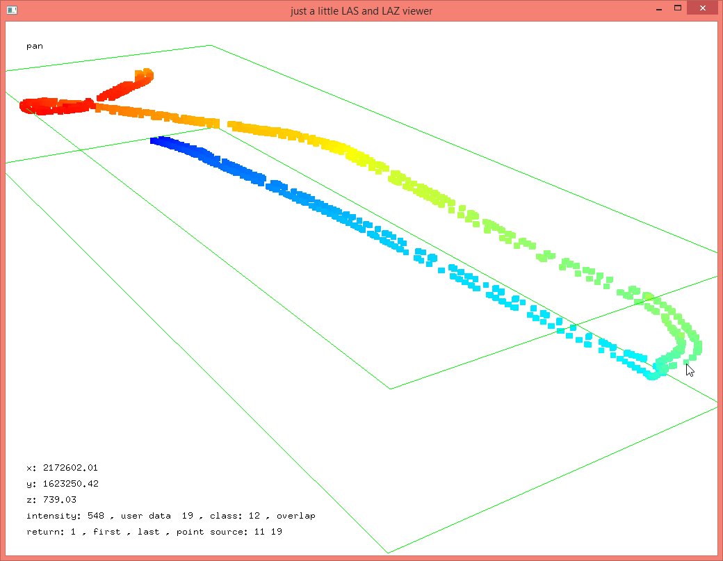Hovering with the mouse over a point that – visually – seems to be one of the turning points of the drone and pressing ‚i‘ on the keyboard shows an intensity value of 548 which corresponds to the GPS time stamp 418548, which we then use to split the LiDAR point cloud (without the trajectory) into two flightlines:

las2las -i Velodyne001_below719.laz ^
        -i Velodyne001_above719_001.laz ^
        -merged ^
        -keep_gps_time_below 418548 ^
        -o flightline1.laz

las2las -i Velodyne001_below719.laz ^
        -i Velodyne001_above719_001.laz ^
        -merged ^
        -keep_gps_time_above 418548 ^
        -o flightline2.laz

Next we use lasoverlap to check how well the LiDAR points from the flight out and the flight back align vertically. This tool computes the difference of the lowest points for each square foot covered by both flightlines. Differences of less than a quarter of a foot are mapped to white, differences of more than half a foot are mapped to saturated red or blue depending on whether the difference is positive or negative:

lasoverlap -i flightline1.laz ^
           -i flightline2.laz ^
           -faf ^
           -min_diff 0.25 -max_diff 0.50 -step 1 ^
           -odir quality -o overlap_025_050.png

We then use a new feature of the LAStools GUI (as of version 180429) to closer inspect larger red or blue areas. We want to use lasmerge and clip out any region that looks suspect for closer examination with lasview. We start the tool in the GUI mode with the ‚-gui‘ command and the two flightlines pre-loaded. Using the new PNG overlay roll-out on the left we add the ‚overlap_025_050_diff.png‘ image from the quality folder created in the last step and clip out three areas.

lasmerge -i flightline1.laz -i flightline2.laz -gui

You can also clip out these three areas using the command lines below:

lasmerge -i flightline1.laz -i flightline2.laz ^
         -faf ^
         -inside 2172500 1623160 2172600 1623165 ^
         -o clip2500_3160_100x005.laz

lasmerge -i flightline1.laz -i flightline2.laz ^
         -faf ^
         -inside 2172450 1623450 2172550 1623455 ^
         -o clip2450_3450_100x005.laz

lasmerge -i flightline1.laz -i flightline2.laz ^
         -faf ^
         -inside 2172430 1623290 2172530 1623310 ^
         -o clip2430_3290_100x020.laz

A closer inspection of the three cut out slices explains the red and blue areas in the difference image created by lasoverlap. We find a small systematic error in two of the slices. In slice ‚clip2500_3160_100x005.laz‚ the green points from flightline 1 are on average slightly higher than the red points from flightline 2. Vice-versa in slice ‚clip2450_3450_100x005.laz‚ the green points from flightline 1 are on average slightly lower than the red points from flightline 2. However, the error is less than half a foot and only happens near the edges of the flightlines. Given that our surfaces are expected to be „fluffy“ anyways (as is typical for Velodyne LiDAR systems), we accept these differences and continue processing.

The strong red and blue colors in the center of the difference image created by lasoverlap is easily explained by looking at slice ‚clip2430_3290_100x020.laz‚. The scanner was „looking“ under a gazebo-like open roof structure from two different directions and therefore always seeing parts of the floor in one flightline that were obscured by the roof in the other.

While working with this data we’ve also implemented a new feature for lastrack that computes the 3D distance between LiDAR points and the trajectory and allows storing the result as an additional per point attribute with extra bytes. Those can then be visualized with lasgrid. Here an example:

lastrack -i flightline1.laz ^
         -i flightline2.laz ^
         -track Velodyne001_above719_012.laz ^
         -store_xyz_range_as_extra_bytes ^
         -odix _xyz_range -olaz ^
         =cores 2

lasgrid -i flightline*_xyz_range.laz -merged ^
        -drop_attribute_below 0 1 ^
        -attribute0 -lowest ^
        -false -set_min_max 20 200 ^
        -o quality/closest_xyz_range_020ft_200ft.png

lasgrid -i flightline*_xyz_range.laz -merged ^
        -drop_attribute_below 0 1 ^
        -attribute0 -highest ^
        -false -set_min_max 30 300 ^
        -o quality/farthest_xyz_range_030ft_300ft.png

Below the complete processing pipeline for creating a median ground model from the „fluffy“ Velodyne LiDAR data that results in the hillshaded DTM shown here. The workflow is similar to those we have developed in earlier blog posts for Velodyne Puck based systems like the Hovermap and the Yellowscan.

lastile -i flightline1.laz ^
        -i flightline2.laz ^
        -faf ^
        -tile_size 250 -buffer 25 -flag_as_withheld ^
        -odir tiles_raw -o somer.laz

lasnoise -i tiles_raw\*.laz ^
         -step_xy 2 -step 1 -isolated 9 ^
         -odir tiles_denoised -olaz ^
          -cores 4

lasthin -i tiles_denoised\*.laz ^
        -ignore_class 7 ^
        -step 1 -percentile 5 10 -classify_as 8 ^
        -odir tiles_thinned_1_foot -olaz ^
        -cores 4

lasthin -i tiles_thinned_1_foot\*.laz ^
        -ignore_class 7 ^
        -step 2 -percentile 5 10 -classify_as 8 ^
        -odir tiles_thinned_2_foot -olaz ^
        -cores 4

lasthin -i tiles_thinned_2_foot\*.laz ^
        -ignore_class 7 ^
        -step 4 -percentile 5 10 -classify_as 8 ^
        -odir tiles_thinned_4_foot -olaz ^
        -cores 4

lasthin -i tiles_thinned_4_foot\*.laz ^
        -ignore_class 7 ^
        -step 8 -percentile 5 10 -classify_as 8 ^
        -odir tiles_thinned_8_foot -olaz ^
        -cores 4

lasground -i tiles_thinned_8_foot\*.laz ^
          -ignore_class 1 7 ^
          -town -extra_fine ^
          -odir tiles_ground_lowest -olaz ^
          -cores 4

lasheight -i tiles_ground_lowest\*.laz ^
          -classify_between -0.05 0.5 6 ^
          -odir tiles_ground_thick -olaz ^
          -cores 4

lasthin -i tiles_ground_thick\*.laz ^
        -ignore_class 1 7 ^
        -step 1 -percentile 50 -classify_as 2 ^
        -odir tiles_ground_median -olaz ^
        -cores 4

las2dem -i tiles_ground_median\*.laz ^
        -keep_class 2 ^
        -step 1 -use_tile_bb ^
        -odir tiles_dtm -obil ^
        -cores 4

blast2dem -i tiles_dtm\*.bil -merged ^
          -step 1 -hillshade ^
          -o dtm_hillshaded.png

We thank Harris Aerial for sharing this LiDAR data set with us flown by their Carrier H4 Hybrid HE drone carrying a Snoopy A series LiDAR system from LidarUSA.